Supported by the China National Science and Technology Major Project. 2017ZX05049-002 Supported by the China National Science and Technology Major Project. 2016ZX05027004-001 the National Natural Science Foundation of China. 41874146 the National Natural Science Foundation of China. 41674130 Fundamental Research Funds for the Central University. 18CX02061A Innovative Fund Project of China National Petroleum Corporation. 2016D-5007-0301 Scientific Research & Technology Development Project of China National Petroleum Corporation. 2017D-3504
Abstract
A linearized rock physics inversion method is proposed to deal with two important issues, rock physical model and inversion algorithm, which restrict the accuracy of rock physics inversion. In this method, first, the complex rock physics model is expanded into Taylor series to get the first-order approximate expression of the inverse problem of rock physics; then the damped least square method is used to solve the linearized rock physics inverse problem directly to get the analytical solution of the rock physics inverse problem. This method does not need global optimization or random sampling, but directly calculates the inverse operation, with high computational efficiency. The theoretical model analysis shows that the linearized rock physical model can be used to approximate the complex rock physics model. The application of actual logging data and seismic data shows that the linearized rock physics inversion method can obtain accurate physical parameters. This method is suitable for linear or slightly non-linear rock physics model, but may not be suitable for highly non-linear rock physics model.
Keywords:rock physics inversion
;
linearization
;
physical parameters
;
rock physics model
;
Taylor expansion
ZHANG Jiajia, YIN Xingyao, ZHANG Guangzhi, GU Yipeng, FAN Xianggang. Prediction method of physical parameters based on linearized rock physics inversion. [J], 2020, 47(1): 59-67 doi:10.1016/S1876-3804(20)60005-2
Introduction
Seismic data contains rich information on seismic elastic properties and reservoir physical parameters[1]. Prediction of reservoir physical parameter usually takes two steps: the first step is to obtain seismic elastic parameters from seismic data using conventional seismic inversion methods. The existent seismic inversion technology is very mature[2,3,4,5], and can obtain quite accurate elastic parameters, such as P- and S-wave velocities and density. The second step is to use rock physics inversion to predict reservoir parameters from seismic elastic parameters, such as porosity, saturation, and shale content[6,7,8]. In rock physics inversion, first, a theoretical or empirical rock physics model needs to be built, that is to work out the relationship between seismic elastic properties and reservoir physical parameters[9,10]; second, the inversion algorithm used in rock physics inversion need to be selected, and currently probability statistical inversion method is used most commonly[11,12].
Both the rock physics model and the rock physics inversion algorithm directly affect the accuracy of reservoir physical parameter inversion. For example, among many rock physics models, the contact cementation model[13] is relatively simple in mathematical form and is widely used in rock physics inversion[14,15]. However, the relationship between elastic properties and physical parameters in actual production is very complicated. For example, the equivalent medium theory is used to establish a rock physics model[16]. If a complex rock physics model is selected, probability statistical inversion algorithms, such as Bayesian method or Monte Carlo algorithm need to be used. Many researchers have carried out a lot of research work in these two aspects. For example, Bachrach et al. established the statistical relationship between physical parameters and elastic parameters, and used Bayesian inversion method to realize the joint inversion of porosity and water saturation[17]. Spikes et al. established the relationship between physical parameters and elastic parameters by using contact cementation model, and used Bayesian inversion to predict porosity, shale content, and water saturation[18]. Bosch used the Wyllie time-average equation[14] and Markov chain Monte Carlo sampling method and least square iterative method to inverse the physical parameters[19]. Deng et al. proposed a Bayesian inversion method based on stochastic rock physics model to realize joint inversion of porosity and water saturation[20]. Grana and Rossa used the contact cementation model[13] for rock physics modeling, and estimated the posterior probability distribution of reservoir parameters under the Bayesian framework to realize the reservoir parameter inversion[21]. Yin et al. established a statistical relationship between the elastic impedance and the physical parameters of the reservoir, and used Bayesian theory to estimate the posterior probability distribution of the physical parameters to realize the inversion of the reservoir physical parameters[11]. Grana proposed a linear approximation of the cemented contact model, used Bayesian theory to solve the rock physics inversion problem and estimate the reservoir physical parameters[22]. Lin et al. used the inclusion model to establish a rock physics model and proposed an inversion method for reservoir physical parameters based on constrained least square and trust region[12]. Li et al. used effective medium theory[23] to construct a three-dimensional rock physics template, and used the least square method of finding the grid points of the three-dimensional template to predict the physical parameters. Yang Peijie established a quantitative relationship between the physical parameters and seismic elastic properties of sand-shale reservoir, and simultaneously inversed the porosity and water saturation of the reservoir based on Bayesian theory[24].
The rock physics models used in the above rock physics inversion methods are relatively simple, such as statistical empirical relationship and cementation contact model. Another issue is that many inversion algorithms use probability statistical inversion algorithms, which require global optimization or random sampling, so the computational efficiency for solving rock physics inverse problems is low. To solve these problems, we have come up with a linearization method of rock physics model. In this method, Taylor expansion of the rock physics model is performed to obtain the first-order approximate expression of the rock physics inverse problem, then the damped least square algorithm is used to directly solve the rock physics inversion problem and obtain the analytical solution. This method doesn’t need global optimization or random sampling, but is direct inversion operation, so it has higher calculation efficiency. In this study, Gassmann equation[25] and critical porosity model[26] were used to build rock physics model of shaly sandstone reservoir. The modeling process is very complicated, and the relationship between the seismic elastic properties and the reservoir physical parameters is non-linear. The actual logging data and seismic data verify that the linearized rock physics inversion method can obtain accurate physical parameters and can be used to approximate the actual rock physics model.
1. Method
1.1. Linearized rock physics inversion
The problem of rock physics inversion can be written as:
d=f(m)
In equation (1), d is the elastic property, m is the physical parameter to be predicted, and f is the relationship between the elastic property and the physical parameter, that is, the rock physics model. For simplicity, first assume that all variables in equation (1) are scalars with a single parameter, and then they are generalized to multiple parameters, for example, d is the P-wave velocity, m is the porosity, and f is the Wyllie time average equation[19] or Raymer's improved equation[27].
In actual production, the rock physics model f is not as simple as Wyllie's time average equation or Raymer's improved equation, and it is often very complicated and nonlinear. Taylor expansion is often used in geophysics to approximate complex non-linear functions, especially in seismic imaging[28]. In order to solve the rock physics inversion problem, a linearized rock physics inversion method based on Taylor expansion is also used in this paper[22].
Taylor expansion is used to linearize the rock physics inversion problem. Here, first-order Taylor expansion is used, then equation (1) can be rewritten as:
$d\cong f(m_{0})+f^{'}(m_{0})(m-m_{0})$
By expanding and merging the polynomials in equation (2), the rock physics inversion problem can be rewritten into a linear form:
Then the linearized rock physics inversion method is extended to multiple parameters, so the elastic property d and the physical parameter m are in the form of vector containing multiple variables. For example, d is a vector composed of elastic properties such as P-wave velocity vp, S-wave velocity vs, and density ρ, and m is a vector composed of physical parameters such as porosity ϕ, water saturation Sw, and shale content C. Similarly, the rock physics model f is also written in vector form, so the rock physics inversion problem can be written as:
d=f(m)
First-order Taylor expansion of equation (4) becomes
$d\cong f(m_{0})+J_{m_{0}}(m-m_{0})$
where $J_{m_{0}}$ is the Jacobian matrix of function f at its argument $m_{0}$ Rewriting it into a linearized form then it becomes:
$d\cong J_{m_{0}}m+(f(m_{0})-J_{m_{0}}m_{0})$
1.2. Rock physics modeling
In this paper, Gassmann equation[25] and critical porosity model[26] are used for rock physics modeling of shaly sandstone. The specific modeling process is as follows:
(1) Bulk modulus $K_{m}$, shear modulus $\mu_{m}$ and density $\rho_{m}$ of rock matrix can be calculated by Voigt-Reuss-Hill average method[29]:
Here the homogeneous mixing model[9] is used to calculate the bulk modulus of the mixed fluid.
(3) Bulk modulus $K_{dry}$ and shear modulus $\mu_{dry}$ of dry rock are calculated using the critical porosity model[26]:
$K_{dry}=K_{m}(1-\frac{\phi}{\phi_{c}})$
$\mu_{dry}=\mu_{m}(1-\frac{\phi}{\phi_{c}})$
Although the critical porosity value $\phi_{c}$ is an empirical value, such as 40% for sandstone and 60% for limestone, etc., the critical porosity value includes the effect of rock pore type or pore shape on P- and S-wave velocities[30].
(4) Bulk modulus $K_{sat}$ and shear modulus $\mu_{sat}$ of saturated rock are calculated by Gassmann equation[25]:
Since the rock physics modeling process, that is, equations (7) to (18) are nonlinear, it can be linearized. The elastic properties d (i.e., P-wave velocity $v_{P}$, S-wave velocity $v_{S}$, and density $\rho$) are differentiated to the physical parameters m (porosity $\phi$, shale volume content $C$, and water saturation $S_{w}$), and the corresponding Jacobian matrix is calculated as:
The partial derivatives of P-wave velocity ${{v}_{\text{P}}}$, S-wave velocity${{v}_{\text{s}}}$, and density $\rho $ to shale content $C$ are very complex, so no specific expression is given in this paper.
The Jacobian matrix is then substituted into the equation (6) of the linearized rock physics inversion problem. There are many ways to solve the linearized rock physics inversion problem, such as the least square algorithm, the damped least square algorithm or the Bayesian method. Here, the damped least square method is used to solve it, and we get:
In order to verify the accuracy of the linearized rock physics inversion, the actual rock physics model and the linearized rock physics model were used to perform rock physics forward modeling of shaly sandstone. Assuming that the the shaly sandstone is made up of quartz and clay, and the pore fluid is a mixture of water and air, the corresponding elastic modulus and density are: ${{K}_{\text{q}}}={{36}_{{}}}\text{GPa}$, ${{\mu }_{\text{q}}}=$ ${{36}_{{}}}\text{GPa}$, ${{\rho }_{\text{q}}}={{2.65}_{{}}}\text{g/c}{{\text{m}}^{\text{3}}}$, ${{K}_{\text{c}}}={{21}_{{}}}\text{GPa}$, ${{\mu }_{\text{c}}}=$ ${{15}_{{}}}\text{GPa}$, ${{\rho }_{\text{c}}}=$2.45 g/cm3, ${{K}_{\text{hc}}}={{0.020}_{{}}}{{8}_{{}}}\text{GPa}$, ${{\rho }_{\text{hc}}}=$ ${{0.001}_{{}}}\text{g/c}{{\text{m}}^{\text{3}}}$, ${{K}_{\text{w}}}=$ 2.25 GPa, ${{\rho }_{\text{w}}}={{1.03}_{{}}}\text{g/c}{{\text{m}}^{\text{3}}}$. The first-order Taylor expansion of linearized rock physics model is performed at the mean of porosity, shale content, and saturation.
Fig. 1. shows the relationships between the elastic propeties (P-wave velocity, S-wave velocity, and density) and porosity. The shale volume content $C$ of the shaly sandstone varies from 0 to 50% at 10% intervals, the saturation ${{S}_{\text{w}}}$ is a constant 30%, and the porosity $\phi $ varies uniformly from 0 to 30%. It can be seen from Fig. 1a and 1b that the linearized rock physics model agree best with the actual rock physics model at the porosity of about 15%, and has some error when the porosity is low and high. This is because the first-order Taylor expansion is performed at the mean porosity of 15%. It can be seen from Fig. 1c that the densities of the linearized rock physics model and the actual rock physics model are exactly the same, this is because the density calculation equation is linear, and the linearized rock physics model is exactly the same as the actual rock physics model.
Fig. 1.
Relationship between elastic properties and porosity calculated by actual rock physics model and linearized rock physics model.
Fig. 2. shows the relationships between the elastic propeties (P-wave velocity, S-wave velocity, and density) and shale content. The porosity $\phi $ of shaly sandstones varies from 0 to 30% at 10% intervals, the water saturation ${{S}_{\text{w}}}$ is a constant 50%, and the shale content $C$ varies uniformly from 0 to 50%. It can be seen from Fig. 2a and 2b that the linearized rock physics model match best with the actual rock physics model at the shale content of 25%, and has some error when the shale content is too low and too high, this is because the first-order Taylor expansion is performed at the mean shale content of 25%. It can also be seen from Fig. 2c that the densities of the linearized rock physics model and the actual rock physics model are exactly the same, because the density calculation equation is linear, and the linearized rock physics model is exactly the same as the actual rock physics model .
Fig. 2.
Relationship between elastic properties and shale content calculated by actual rock physics model and linearized rock physics model.
Fig. 3 shows the relationships between the elastic propeties (P-wave velocity, S-wave velocity, and density) and water saturation. The porosity $\phi $ of shaly sandstone varies from 0 to 30% at the interval of 10%, the shale content $C$ is a constant of 25%, and the water saturation ${{S}_{\text{w}}}$ varies uniformly from 0 to 100%. It can be seen from Fig. 3a and 3b that by using bulk modulus of the mixed fluid calculated by the homogeous mixing equation, the P-wave velocity worked out by the linearized rock physics model agrees well with that by the actual rock physics model, has larger error only when the water saturation ${{S}_{\text{w}}}$ is close to 100% and meets the approximate requirements. It can also be seen from Fig. 3c that the densities of the linearized rock physics model and the actual rock physics model are exactly the same, because the density calculation equation is linear, and the linearized rock physics model is exactly the same as the actual rock physics model.
Fig. 3.
Relationship between elastic properties and water saturation calculated by actual rock physics model and linearized rock physics model.
2. Practical application
2.1. Comparison of well logging data
First the linearized rock physics inversion method was applied to actual well logging data. Well A is located in an offshore oil field in eastern China. The reservoir is gas-bearing sandstone. The logging curves include physical parameters such as porosity, shale content and water saturation, as well as elastic properties such as P-wave velocity, S-wave velocity and density (Fig. 4). The well logging data was converted from the depth domain to the time domain after well-seismic calibration, and was resampled at the rate of 2 ms. The major gas pay is a set of thick sandstone reservoir with a time depth of 2 760-2 800 ms. It is overlaid with a thin mudstone layer at about 2 718 ms. There is a thin set of sandstone at 2 810-2 822 ms, below this layer is a set of thick mudstone.
Before performing linearized rock physics inversion, we first made forward modeling. The shaly sandstone is composed of quartz and clay, and the pore fluid is a mixture of water and gas. The corresponding elastic modulus and density are: ${{K}_{\text{q}}}={{38}_{{}}}\text{GPa}$, ${{\mu }_{\text{q}}}={{40}_{{}}}\text{GPa}$, ${{\rho }_{\text{q}}}={{2.65}_{{}}}\text{g/c}{{\text{m}}^{\text{3}}}$, ${{K}_{\text{c}}}=$15 GPa, ${{\mu }_{\text{c}}}={{7}_{{}}}\text{GPa}$, ${{\rho }_{\text{c}}}={{2.55}_{{}}}\text{g/c}{{\text{m}}^{\text{3}}}$, ${{K}_{\text{hc}}}=$ ${{0.020}_{{}}}{{8}_{{}}}\text{GPa}$,${{\rho }_{\text{hc}}}={{0.001}_{{}}}\text{g/c}{{\text{m}}^{\text{3}}}$,${{K}_{\text{w}}}={{2.25}_{{}}}\text{GPa}$,${{\rho }_{\text{w}}}=$ ${{1.03}_{{}}}\text{g/c}{{\text{m}}^{\text{3}}}$. By using accurate rock physics model and linearized rock physics model, the P- and S-wave velocities and density in Fig. 5 were calculated from the physical parameters such as porosity, shale content and water saturation in Fig. 4. The solid blue line in the Fig. 5 represents the actual logging data, the solid black line represents the forward modeling result of the actual rock physics model, and the red dashed line represents the forward modeling result of the linear rock physics model. It can be seen from Fig. 5 that the forward modeling results from the linearized rock physics model are basically the same with the results from the actual rock physics model, and have some error but the same change trend with the actual logging curve. The average errors between the P-wave velocity, S-wave velocity and density calculated from linearized rock physics model and the actual P-wave velocity, S-wave velocity and density are about 4.0%, 3.0%, and 1.2% respectively. The errors of the mudstone section between 2 820 and 2 860 ms are larger, mainly because the elastic modulus of the mudstone varies greatly, and it is difficult to obtain accurate value.
Fig. 5.
Elastic properties calculated from forward modeling of actual rock physics model and linearized rock physics model, and actual well logging data.
Secondly, linearized rock physics inversion was performed on the logging data, that is, the porosity, shale content, and water saturation in Fig. 4a-4c were inversely modeled using the P-wave velocity, S-wave velocity, and density in Fig. 4d-4f. Parameters such as elastic modulus and density used were the same as those in Fig. 5, and the inversion results are shown in Fig. 6. It can be seen from Fig. 6 that the inversion results from the linearized rock physics model are basically consistent with the actual log curves. Although the amplitudes do not exactly match, the overall trend is the same. The porosity, water saturation and shale content from inversion have correlation coefficients of 64.8%, 85.4% and 90.2% and average errors of about 28%, 17% and 10% with the corresponding porosity, water saturation and shale content from actual log.
Fig. 6.
Physical parameters from inversion with linearized rock physics model and actual well logging data.
2.2. Comparison of seismic data
After the rock physics inversion of the well logging data, the seismic data was inversely modeled with the linearized rock physics model. A two-dimensional seismic profile through Well A was selected, and two-dimensional profiles of elastic properties such as P-wave velocity, S-wave velocity, and density were obtained from simultaneous prestack inversion[31] (Fig. 7). From the two-dimensional elastic parameter profiles, it can be seen that the P-wave velocity, S-wave velocity, and density all have a low-value section around 2 800 ms, which is the main target reservoir.
Fig. 7.
Profiles of elastic properties from inversion.
Then the elastic properties in Fig. 7 were used to obtain the physical parameters from inversion (Fig. 8). Fig. 8a-8c show the results of porosity, shale content, and gas saturation obtained by linearized rock physics inversion. Fig. 8d-8f shows the fitting results of porosity, shale content, and gas saturation obtained by the empirical relationships between the elastic properties and physical parameters. It can be seen from the inversion results that the physical parameters of the main target reservoir obtained by the two inversion results are in good agreement with the actual parameters on Well A, and the spatial distribution of the physical parameters of the main target reservoir can be obtained. Especially the gas saturation results from linearized rock physics inversion are better than the fitting results from empirical relationship.
Fig. 8.
Physical parameters from linearized rock physics inversion and empirical relationship fitting.
3. Discussion
This paper presents a linearized rock physics inversion method. Because rock physics models aren’t linear usually, this method is more suitable for rock physics models that are not highly non-linear, especially for reservoirs with simple pore structures, such as clastic reservoirs, but isn’t very suitable for reservoirs with complex pore structures, such as carbonate reservoirs. In addition, it is also worth noting that different rock physics models should be slected for different rock types. In this study, we chose critical porosity model and Gassmann equation for modeling the shaly sandstone reservoir, which is reasonable. For other types of reservoirs, other rock physics models are needed. The forward rock physics modeling reslults in this study shows that the linearized rock physics model can be approximated as the the actual rock physics model. The advantage of using a linearized rock physics model is that the analytical solution of the rock physics inverse problem can be obtained. In this study, the damped least square method was taken to solve the linear inversion problem, which is fast in computation, but is sensitive to parameters such as elastic modulus and density used in rock physics modeling. In addition, unlike other rock physics inversion methods, the shale content and saturation obtained by linearized rock physics inversion method have higher accuracy than porosity. The main reason is that in the inverse of the Jacobian matrix, the coefficient terms related to shale content and saturation are larger, while the coefficient terms related to porosity are smaller. Of course, the elastic properties in this work were obtained by AVO prestack seismic inversion. In the next step, we can directly use seismic data to perform rock physics inversion.
4. Conclusions
A linearized rock physics inversion method is proposed, that is, a first-order approximate linearized rock physics model is obtained by Taylor series expansion of the actual rock physics model, then the damped least square method is adopted to solve the linearized rock physics inversion problem to get accurate analytical solutions. The Gassmann equation and critical porosity model were used to build rock physics model of shaly sandstone, and their linearized rock physics model expressions were given. This method is suitable for linear or slightly nonlinear rock physics models, and may not be suitable for highly nonlinear rock physics models. The application on actual logging data and seismic data shows that the linearized rock physics inversion method can obtain quite accurate physical parameter results.
Nomenclature
$C$—shale content, %;
C0—mean of shale content, %;
d—elastic property;
d—vector of elastic property;
f—rock physics model;
${f}'$—first derivative of rock physics model;
$\mathbf{f}$—vector of rock physics model;
$\mathbf{f}\left( {{\mathbf{m}}_{0}} \right)$—value of rock physics model at ${{\mathbf{m}}_{0}}$=(${{\phi }_{0}}$,${{C}_{0}}$,${{S}_{\text{w0}}}$);
$\mathbf{I}$—identity matrix;
${{\mathbf{J}}_{{{\mathbf{m}}_{\text{0}}}}}$—value of Jacobian matrix at ${{\mathbf{m}}_{0}}$=(${{\phi }_{0}}$,${{C}_{0}}$,${{S}_{\text{w0}}}$);
${{K}_{\text{c}}}$—bulk modulus of clay minerals, GPa;
${{K}_{\text{dry}}}$—bulk modulus of dry rock, GPa;
${{K}_{\text{fl}}}$—bulk modulus of mixed fluid, GPa;
${{K}_{\text{m}}}$—bulk modulus of rock matrix, GPa;
${{K}_{\text{hc}}}$—bulk modulus of hydrocarbons such as oil or gas, GPa;
${{K}_{\text{q}}}$—bulk modulus of sandy minerals, GPa;
${{K}_{\text{sat}}}$—bulk modulus of saturated rock, GPa;
${{K}_{\text{w}}}$—bulk modulus of water, GPa;
m—physical parameter to be predicted;
${{m}_{0}}$—specific value of the physical parameter m, ${{m}_{0}}$ is often selected as the mean value of the model parameter to be predicted;
$\mathbf{m}$—vector of the physical parameter to be predicted;
${{\mathbf{m}}_{\text{0}}}$—specific value of physical parameter vector $\mathbf{m}$, ${{\mathbf{m}}_{\text{0}}}$=(${{\phi }_{0}}$, ${{C}_{0}}$,${{S}_{\text{w0}}}$);
${{S}_{\text{w}}}$—water saturation, %;
${{S}_{\text{w0}}}$—mean of water saturation, %;
${{v}_{\text{P}}}$—P-wave velocity of saturated rock, km/s;
${{v}_{\operatorname{S}}}$—S-wave velocity of saturated rock, km/s;
$\rho $—density of saturated rock, g/cm3;
${{\rho }_{\text{c}}}$—density of mineral, g/cm3;
${{\rho }_{\text{fl}}}$—density of saturation fluid, g/cm3;
${{\rho }_{\text{hc}}}$—density of hydrocarbons such as oil or gas, g/cm3;
${{\rho }_{\text{m}}}$—density of rock matrix, g/cm3;
${{\rho }_{\text{q}}}$—density of sandy minerals, g/cm3;
${{\rho }_{\operatorname{w}}}$—density of water, g/cm3;
$\phi $—porosity, %;
${{\phi }_{0}}$—mean of porosity, %;
${{\phi }_{\text{c}}}$—critical porosity of rock, %;
${{\mu }_{\text{c}}}$—shear modulus of clay minerals, GPa;
${{\mu }_{\text{dry}}}$—shear modulus of dry rock, GPa;
${{\mu }_{\text{m}}}$—shear modulus of rock matrix, GPa;
${{\mu }_{\text{q}}}$—shear modulus of sandy minerals, GPa;
${{\mu }_{\text{sat}}}$—shear modulus of saturated rock, GPa;
A permeability prediction method based on pore structure and lithofacies
1
2019
... Seismic data contains rich information on seismic elastic properties and reservoir physical parameters[1]. Prediction of reservoir physical parameter usually takes two steps: the first step is to obtain seismic elastic parameters from seismic data using conventional seismic inversion methods. The existent seismic inversion technology is very mature[2,3,4,5], and can obtain quite accurate elastic parameters, such as P- and S-wave velocities and density. The second step is to use rock physics inversion to predict reservoir parameters from seismic elastic parameters, such as porosity, saturation, and shale content[6,7,8]. In rock physics inversion, first, a theoretical or empirical rock physics model needs to be built, that is to work out the relationship between seismic elastic properties and reservoir physical parameters[9,10]; second, the inversion algorithm used in rock physics inversion need to be selected, and currently probability statistical inversion method is used most commonly[11,12]. ...
Elastic impedance
1
1999
... Seismic data contains rich information on seismic elastic properties and reservoir physical parameters[1]. Prediction of reservoir physical parameter usually takes two steps: the first step is to obtain seismic elastic parameters from seismic data using conventional seismic inversion methods. The existent seismic inversion technology is very mature[2,3,4,5], and can obtain quite accurate elastic parameters, such as P- and S-wave velocities and density. The second step is to use rock physics inversion to predict reservoir parameters from seismic elastic parameters, such as porosity, saturation, and shale content[6,7,8]. In rock physics inversion, first, a theoretical or empirical rock physics model needs to be built, that is to work out the relationship between seismic elastic properties and reservoir physical parameters[9,10]; second, the inversion algorithm used in rock physics inversion need to be selected, and currently probability statistical inversion method is used most commonly[11,12]. ...
Introduction to seismic inversion methods
1
1988
... Seismic data contains rich information on seismic elastic properties and reservoir physical parameters[1]. Prediction of reservoir physical parameter usually takes two steps: the first step is to obtain seismic elastic parameters from seismic data using conventional seismic inversion methods. The existent seismic inversion technology is very mature[2,3,4,5], and can obtain quite accurate elastic parameters, such as P- and S-wave velocities and density. The second step is to use rock physics inversion to predict reservoir parameters from seismic elastic parameters, such as porosity, saturation, and shale content[6,7,8]. In rock physics inversion, first, a theoretical or empirical rock physics model needs to be built, that is to work out the relationship between seismic elastic properties and reservoir physical parameters[9,10]; second, the inversion algorithm used in rock physics inversion need to be selected, and currently probability statistical inversion method is used most commonly[11,12]. ...
Seismic prediction method of pore fluid in tight gas reservoirs, Ordos Basin, NW China
1
2017
... Seismic data contains rich information on seismic elastic properties and reservoir physical parameters[1]. Prediction of reservoir physical parameter usually takes two steps: the first step is to obtain seismic elastic parameters from seismic data using conventional seismic inversion methods. The existent seismic inversion technology is very mature[2,3,4,5], and can obtain quite accurate elastic parameters, such as P- and S-wave velocities and density. The second step is to use rock physics inversion to predict reservoir parameters from seismic elastic parameters, such as porosity, saturation, and shale content[6,7,8]. In rock physics inversion, first, a theoretical or empirical rock physics model needs to be built, that is to work out the relationship between seismic elastic properties and reservoir physical parameters[9,10]; second, the inversion algorithm used in rock physics inversion need to be selected, and currently probability statistical inversion method is used most commonly[11,12]. ...
Quantitative seismic prediction of shale gas sweet spots in Lower Silurian Longmaxi Formation, Weiyuan area, Sichuan Basin, SW China
1
2018
... Seismic data contains rich information on seismic elastic properties and reservoir physical parameters[1]. Prediction of reservoir physical parameter usually takes two steps: the first step is to obtain seismic elastic parameters from seismic data using conventional seismic inversion methods. The existent seismic inversion technology is very mature[2,3,4,5], and can obtain quite accurate elastic parameters, such as P- and S-wave velocities and density. The second step is to use rock physics inversion to predict reservoir parameters from seismic elastic parameters, such as porosity, saturation, and shale content[6,7,8]. In rock physics inversion, first, a theoretical or empirical rock physics model needs to be built, that is to work out the relationship between seismic elastic properties and reservoir physical parameters[9,10]; second, the inversion algorithm used in rock physics inversion need to be selected, and currently probability statistical inversion method is used most commonly[11,12]. ...
Predicting shale and porosity using cascaded seismic and rock physics inversion
1
2005
... Seismic data contains rich information on seismic elastic properties and reservoir physical parameters[1]. Prediction of reservoir physical parameter usually takes two steps: the first step is to obtain seismic elastic parameters from seismic data using conventional seismic inversion methods. The existent seismic inversion technology is very mature[2,3,4,5], and can obtain quite accurate elastic parameters, such as P- and S-wave velocities and density. The second step is to use rock physics inversion to predict reservoir parameters from seismic elastic parameters, such as porosity, saturation, and shale content[6,7,8]. In rock physics inversion, first, a theoretical or empirical rock physics model needs to be built, that is to work out the relationship between seismic elastic properties and reservoir physical parameters[9,10]; second, the inversion algorithm used in rock physics inversion need to be selected, and currently probability statistical inversion method is used most commonly[11,12]. ...
Seismic reservoir characterization: An earth modelling perspective
1
2007
... Seismic data contains rich information on seismic elastic properties and reservoir physical parameters[1]. Prediction of reservoir physical parameter usually takes two steps: the first step is to obtain seismic elastic parameters from seismic data using conventional seismic inversion methods. The existent seismic inversion technology is very mature[2,3,4,5], and can obtain quite accurate elastic parameters, such as P- and S-wave velocities and density. The second step is to use rock physics inversion to predict reservoir parameters from seismic elastic parameters, such as porosity, saturation, and shale content[6,7,8]. In rock physics inversion, first, a theoretical or empirical rock physics model needs to be built, that is to work out the relationship between seismic elastic properties and reservoir physical parameters[9,10]; second, the inversion algorithm used in rock physics inversion need to be selected, and currently probability statistical inversion method is used most commonly[11,12]. ...
Joint inversion of petrophysical parameters based on Bayesian classification
1
2012
... Seismic data contains rich information on seismic elastic properties and reservoir physical parameters[1]. Prediction of reservoir physical parameter usually takes two steps: the first step is to obtain seismic elastic parameters from seismic data using conventional seismic inversion methods. The existent seismic inversion technology is very mature[2,3,4,5], and can obtain quite accurate elastic parameters, such as P- and S-wave velocities and density. The second step is to use rock physics inversion to predict reservoir parameters from seismic elastic parameters, such as porosity, saturation, and shale content[6,7,8]. In rock physics inversion, first, a theoretical or empirical rock physics model needs to be built, that is to work out the relationship between seismic elastic properties and reservoir physical parameters[9,10]; second, the inversion algorithm used in rock physics inversion need to be selected, and currently probability statistical inversion method is used most commonly[11,12]. ...
2
2009
... Seismic data contains rich information on seismic elastic properties and reservoir physical parameters[1]. Prediction of reservoir physical parameter usually takes two steps: the first step is to obtain seismic elastic parameters from seismic data using conventional seismic inversion methods. The existent seismic inversion technology is very mature[2,3,4,5], and can obtain quite accurate elastic parameters, such as P- and S-wave velocities and density. The second step is to use rock physics inversion to predict reservoir parameters from seismic elastic parameters, such as porosity, saturation, and shale content[6,7,8]. In rock physics inversion, first, a theoretical or empirical rock physics model needs to be built, that is to work out the relationship between seismic elastic properties and reservoir physical parameters[9,10]; second, the inversion algorithm used in rock physics inversion need to be selected, and currently probability statistical inversion method is used most commonly[11,12]. ...
... Here the homogeneous mixing model[9] is used to calculate the bulk modulus of the mixed fluid. ...
1
2005
... Seismic data contains rich information on seismic elastic properties and reservoir physical parameters[1]. Prediction of reservoir physical parameter usually takes two steps: the first step is to obtain seismic elastic parameters from seismic data using conventional seismic inversion methods. The existent seismic inversion technology is very mature[2,3,4,5], and can obtain quite accurate elastic parameters, such as P- and S-wave velocities and density. The second step is to use rock physics inversion to predict reservoir parameters from seismic elastic parameters, such as porosity, saturation, and shale content[6,7,8]. In rock physics inversion, first, a theoretical or empirical rock physics model needs to be built, that is to work out the relationship between seismic elastic properties and reservoir physical parameters[9,10]; second, the inversion algorithm used in rock physics inversion need to be selected, and currently probability statistical inversion method is used most commonly[11,12]. ...
Petrophysical property inversion of reservoirs based on elastic impedance
2
2014
... Seismic data contains rich information on seismic elastic properties and reservoir physical parameters[1]. Prediction of reservoir physical parameter usually takes two steps: the first step is to obtain seismic elastic parameters from seismic data using conventional seismic inversion methods. The existent seismic inversion technology is very mature[2,3,4,5], and can obtain quite accurate elastic parameters, such as P- and S-wave velocities and density. The second step is to use rock physics inversion to predict reservoir parameters from seismic elastic parameters, such as porosity, saturation, and shale content[6,7,8]. In rock physics inversion, first, a theoretical or empirical rock physics model needs to be built, that is to work out the relationship between seismic elastic properties and reservoir physical parameters[9,10]; second, the inversion algorithm used in rock physics inversion need to be selected, and currently probability statistical inversion method is used most commonly[11,12]. ...
... Both the rock physics model and the rock physics inversion algorithm directly affect the accuracy of reservoir physical parameter inversion. For example, among many rock physics models, the contact cementation model[13] is relatively simple in mathematical form and is widely used in rock physics inversion[14,15]. However, the relationship between elastic properties and physical parameters in actual production is very complicated. For example, the equivalent medium theory is used to establish a rock physics model[16]. If a complex rock physics model is selected, probability statistical inversion algorithms, such as Bayesian method or Monte Carlo algorithm need to be used. Many researchers have carried out a lot of research work in these two aspects. For example, Bachrach et al. established the statistical relationship between physical parameters and elastic parameters, and used Bayesian inversion method to realize the joint inversion of porosity and water saturation[17]. Spikes et al. established the relationship between physical parameters and elastic parameters by using contact cementation model, and used Bayesian inversion to predict porosity, shale content, and water saturation[18]. Bosch used the Wyllie time-average equation[14] and Markov chain Monte Carlo sampling method and least square iterative method to inverse the physical parameters[19]. Deng et al. proposed a Bayesian inversion method based on stochastic rock physics model to realize joint inversion of porosity and water saturation[20]. Grana and Rossa used the contact cementation model[13] for rock physics modeling, and estimated the posterior probability distribution of reservoir parameters under the Bayesian framework to realize the reservoir parameter inversion[21]. Yin et al. established a statistical relationship between the elastic impedance and the physical parameters of the reservoir, and used Bayesian theory to estimate the posterior probability distribution of the physical parameters to realize the inversion of the reservoir physical parameters[11]. Grana proposed a linear approximation of the cemented contact model, used Bayesian theory to solve the rock physics inversion problem and estimate the reservoir physical parameters[22]. Lin et al. used the inclusion model to establish a rock physics model and proposed an inversion method for reservoir physical parameters based on constrained least square and trust region[12]. Li et al. used effective medium theory[23] to construct a three-dimensional rock physics template, and used the least square method of finding the grid points of the three-dimensional template to predict the physical parameters. Yang Peijie established a quantitative relationship between the physical parameters and seismic elastic properties of sand-shale reservoir, and simultaneously inversed the porosity and water saturation of the reservoir based on Bayesian theory[24]. ...
The petrophysical parameter inversion method based on constrained least squares and trust region approach
2
2017
... Seismic data contains rich information on seismic elastic properties and reservoir physical parameters[1]. Prediction of reservoir physical parameter usually takes two steps: the first step is to obtain seismic elastic parameters from seismic data using conventional seismic inversion methods. The existent seismic inversion technology is very mature[2,3,4,5], and can obtain quite accurate elastic parameters, such as P- and S-wave velocities and density. The second step is to use rock physics inversion to predict reservoir parameters from seismic elastic parameters, such as porosity, saturation, and shale content[6,7,8]. In rock physics inversion, first, a theoretical or empirical rock physics model needs to be built, that is to work out the relationship between seismic elastic properties and reservoir physical parameters[9,10]; second, the inversion algorithm used in rock physics inversion need to be selected, and currently probability statistical inversion method is used most commonly[11,12]. ...
... Both the rock physics model and the rock physics inversion algorithm directly affect the accuracy of reservoir physical parameter inversion. For example, among many rock physics models, the contact cementation model[13] is relatively simple in mathematical form and is widely used in rock physics inversion[14,15]. However, the relationship between elastic properties and physical parameters in actual production is very complicated. For example, the equivalent medium theory is used to establish a rock physics model[16]. If a complex rock physics model is selected, probability statistical inversion algorithms, such as Bayesian method or Monte Carlo algorithm need to be used. Many researchers have carried out a lot of research work in these two aspects. For example, Bachrach et al. established the statistical relationship between physical parameters and elastic parameters, and used Bayesian inversion method to realize the joint inversion of porosity and water saturation[17]. Spikes et al. established the relationship between physical parameters and elastic parameters by using contact cementation model, and used Bayesian inversion to predict porosity, shale content, and water saturation[18]. Bosch used the Wyllie time-average equation[14] and Markov chain Monte Carlo sampling method and least square iterative method to inverse the physical parameters[19]. Deng et al. proposed a Bayesian inversion method based on stochastic rock physics model to realize joint inversion of porosity and water saturation[20]. Grana and Rossa used the contact cementation model[13] for rock physics modeling, and estimated the posterior probability distribution of reservoir parameters under the Bayesian framework to realize the reservoir parameter inversion[21]. Yin et al. established a statistical relationship between the elastic impedance and the physical parameters of the reservoir, and used Bayesian theory to estimate the posterior probability distribution of the physical parameters to realize the inversion of the reservoir physical parameters[11]. Grana proposed a linear approximation of the cemented contact model, used Bayesian theory to solve the rock physics inversion problem and estimate the reservoir physical parameters[22]. Lin et al. used the inclusion model to establish a rock physics model and proposed an inversion method for reservoir physical parameters based on constrained least square and trust region[12]. Li et al. used effective medium theory[23] to construct a three-dimensional rock physics template, and used the least square method of finding the grid points of the three-dimensional template to predict the physical parameters. Yang Peijie established a quantitative relationship between the physical parameters and seismic elastic properties of sand-shale reservoir, and simultaneously inversed the porosity and water saturation of the reservoir based on Bayesian theory[24]. ...
Effective properties of cemented granular materials
2
1994
... Both the rock physics model and the rock physics inversion algorithm directly affect the accuracy of reservoir physical parameter inversion. For example, among many rock physics models, the contact cementation model[13] is relatively simple in mathematical form and is widely used in rock physics inversion[14,15]. However, the relationship between elastic properties and physical parameters in actual production is very complicated. For example, the equivalent medium theory is used to establish a rock physics model[16]. If a complex rock physics model is selected, probability statistical inversion algorithms, such as Bayesian method or Monte Carlo algorithm need to be used. Many researchers have carried out a lot of research work in these two aspects. For example, Bachrach et al. established the statistical relationship between physical parameters and elastic parameters, and used Bayesian inversion method to realize the joint inversion of porosity and water saturation[17]. Spikes et al. established the relationship between physical parameters and elastic parameters by using contact cementation model, and used Bayesian inversion to predict porosity, shale content, and water saturation[18]. Bosch used the Wyllie time-average equation[14] and Markov chain Monte Carlo sampling method and least square iterative method to inverse the physical parameters[19]. Deng et al. proposed a Bayesian inversion method based on stochastic rock physics model to realize joint inversion of porosity and water saturation[20]. Grana and Rossa used the contact cementation model[13] for rock physics modeling, and estimated the posterior probability distribution of reservoir parameters under the Bayesian framework to realize the reservoir parameter inversion[21]. Yin et al. established a statistical relationship between the elastic impedance and the physical parameters of the reservoir, and used Bayesian theory to estimate the posterior probability distribution of the physical parameters to realize the inversion of the reservoir physical parameters[11]. Grana proposed a linear approximation of the cemented contact model, used Bayesian theory to solve the rock physics inversion problem and estimate the reservoir physical parameters[22]. Lin et al. used the inclusion model to establish a rock physics model and proposed an inversion method for reservoir physical parameters based on constrained least square and trust region[12]. Li et al. used effective medium theory[23] to construct a three-dimensional rock physics template, and used the least square method of finding the grid points of the three-dimensional template to predict the physical parameters. Yang Peijie established a quantitative relationship between the physical parameters and seismic elastic properties of sand-shale reservoir, and simultaneously inversed the porosity and water saturation of the reservoir based on Bayesian theory[24]. ...
... [13] for rock physics modeling, and estimated the posterior probability distribution of reservoir parameters under the Bayesian framework to realize the reservoir parameter inversion[21]. Yin et al. established a statistical relationship between the elastic impedance and the physical parameters of the reservoir, and used Bayesian theory to estimate the posterior probability distribution of the physical parameters to realize the inversion of the reservoir physical parameters[11]. Grana proposed a linear approximation of the cemented contact model, used Bayesian theory to solve the rock physics inversion problem and estimate the reservoir physical parameters[22]. Lin et al. used the inclusion model to establish a rock physics model and proposed an inversion method for reservoir physical parameters based on constrained least square and trust region[12]. Li et al. used effective medium theory[23] to construct a three-dimensional rock physics template, and used the least square method of finding the grid points of the three-dimensional template to predict the physical parameters. Yang Peijie established a quantitative relationship between the physical parameters and seismic elastic properties of sand-shale reservoir, and simultaneously inversed the porosity and water saturation of the reservoir based on Bayesian theory[24]. ...
Petrophysical seismic inversion conditioned to well-log data: Methods and application to a gas reservoir
2
2009
... Both the rock physics model and the rock physics inversion algorithm directly affect the accuracy of reservoir physical parameter inversion. For example, among many rock physics models, the contact cementation model[13] is relatively simple in mathematical form and is widely used in rock physics inversion[14,15]. However, the relationship between elastic properties and physical parameters in actual production is very complicated. For example, the equivalent medium theory is used to establish a rock physics model[16]. If a complex rock physics model is selected, probability statistical inversion algorithms, such as Bayesian method or Monte Carlo algorithm need to be used. Many researchers have carried out a lot of research work in these two aspects. For example, Bachrach et al. established the statistical relationship between physical parameters and elastic parameters, and used Bayesian inversion method to realize the joint inversion of porosity and water saturation[17]. Spikes et al. established the relationship between physical parameters and elastic parameters by using contact cementation model, and used Bayesian inversion to predict porosity, shale content, and water saturation[18]. Bosch used the Wyllie time-average equation[14] and Markov chain Monte Carlo sampling method and least square iterative method to inverse the physical parameters[19]. Deng et al. proposed a Bayesian inversion method based on stochastic rock physics model to realize joint inversion of porosity and water saturation[20]. Grana and Rossa used the contact cementation model[13] for rock physics modeling, and estimated the posterior probability distribution of reservoir parameters under the Bayesian framework to realize the reservoir parameter inversion[21]. Yin et al. established a statistical relationship between the elastic impedance and the physical parameters of the reservoir, and used Bayesian theory to estimate the posterior probability distribution of the physical parameters to realize the inversion of the reservoir physical parameters[11]. Grana proposed a linear approximation of the cemented contact model, used Bayesian theory to solve the rock physics inversion problem and estimate the reservoir physical parameters[22]. Lin et al. used the inclusion model to establish a rock physics model and proposed an inversion method for reservoir physical parameters based on constrained least square and trust region[12]. Li et al. used effective medium theory[23] to construct a three-dimensional rock physics template, and used the least square method of finding the grid points of the three-dimensional template to predict the physical parameters. Yang Peijie established a quantitative relationship between the physical parameters and seismic elastic properties of sand-shale reservoir, and simultaneously inversed the porosity and water saturation of the reservoir based on Bayesian theory[24]. ...
... [14] and Markov chain Monte Carlo sampling method and least square iterative method to inverse the physical parameters[19]. Deng et al. proposed a Bayesian inversion method based on stochastic rock physics model to realize joint inversion of porosity and water saturation[20]. Grana and Rossa used the contact cementation model[13] for rock physics modeling, and estimated the posterior probability distribution of reservoir parameters under the Bayesian framework to realize the reservoir parameter inversion[21]. Yin et al. established a statistical relationship between the elastic impedance and the physical parameters of the reservoir, and used Bayesian theory to estimate the posterior probability distribution of the physical parameters to realize the inversion of the reservoir physical parameters[11]. Grana proposed a linear approximation of the cemented contact model, used Bayesian theory to solve the rock physics inversion problem and estimate the reservoir physical parameters[22]. Lin et al. used the inclusion model to establish a rock physics model and proposed an inversion method for reservoir physical parameters based on constrained least square and trust region[12]. Li et al. used effective medium theory[23] to construct a three-dimensional rock physics template, and used the least square method of finding the grid points of the three-dimensional template to predict the physical parameters. Yang Peijie established a quantitative relationship between the physical parameters and seismic elastic properties of sand-shale reservoir, and simultaneously inversed the porosity and water saturation of the reservoir based on Bayesian theory[24]. ...
Bayesian inversion methods for seismic reservoir characterization and time-lapse studies
1
2013
... Both the rock physics model and the rock physics inversion algorithm directly affect the accuracy of reservoir physical parameter inversion. For example, among many rock physics models, the contact cementation model[13] is relatively simple in mathematical form and is widely used in rock physics inversion[14,15]. However, the relationship between elastic properties and physical parameters in actual production is very complicated. For example, the equivalent medium theory is used to establish a rock physics model[16]. If a complex rock physics model is selected, probability statistical inversion algorithms, such as Bayesian method or Monte Carlo algorithm need to be used. Many researchers have carried out a lot of research work in these two aspects. For example, Bachrach et al. established the statistical relationship between physical parameters and elastic parameters, and used Bayesian inversion method to realize the joint inversion of porosity and water saturation[17]. Spikes et al. established the relationship between physical parameters and elastic parameters by using contact cementation model, and used Bayesian inversion to predict porosity, shale content, and water saturation[18]. Bosch used the Wyllie time-average equation[14] and Markov chain Monte Carlo sampling method and least square iterative method to inverse the physical parameters[19]. Deng et al. proposed a Bayesian inversion method based on stochastic rock physics model to realize joint inversion of porosity and water saturation[20]. Grana and Rossa used the contact cementation model[13] for rock physics modeling, and estimated the posterior probability distribution of reservoir parameters under the Bayesian framework to realize the reservoir parameter inversion[21]. Yin et al. established a statistical relationship between the elastic impedance and the physical parameters of the reservoir, and used Bayesian theory to estimate the posterior probability distribution of the physical parameters to realize the inversion of the reservoir physical parameters[11]. Grana proposed a linear approximation of the cemented contact model, used Bayesian theory to solve the rock physics inversion problem and estimate the reservoir physical parameters[22]. Lin et al. used the inclusion model to establish a rock physics model and proposed an inversion method for reservoir physical parameters based on constrained least square and trust region[12]. Li et al. used effective medium theory[23] to construct a three-dimensional rock physics template, and used the least square method of finding the grid points of the three-dimensional template to predict the physical parameters. Yang Peijie established a quantitative relationship between the physical parameters and seismic elastic properties of sand-shale reservoir, and simultaneously inversed the porosity and water saturation of the reservoir based on Bayesian theory[24]. ...
A differential effective medium model of multiple-porosity rock and its analytical approximations for dry rock
1
2014
... Both the rock physics model and the rock physics inversion algorithm directly affect the accuracy of reservoir physical parameter inversion. For example, among many rock physics models, the contact cementation model[13] is relatively simple in mathematical form and is widely used in rock physics inversion[14,15]. However, the relationship between elastic properties and physical parameters in actual production is very complicated. For example, the equivalent medium theory is used to establish a rock physics model[16]. If a complex rock physics model is selected, probability statistical inversion algorithms, such as Bayesian method or Monte Carlo algorithm need to be used. Many researchers have carried out a lot of research work in these two aspects. For example, Bachrach et al. established the statistical relationship between physical parameters and elastic parameters, and used Bayesian inversion method to realize the joint inversion of porosity and water saturation[17]. Spikes et al. established the relationship between physical parameters and elastic parameters by using contact cementation model, and used Bayesian inversion to predict porosity, shale content, and water saturation[18]. Bosch used the Wyllie time-average equation[14] and Markov chain Monte Carlo sampling method and least square iterative method to inverse the physical parameters[19]. Deng et al. proposed a Bayesian inversion method based on stochastic rock physics model to realize joint inversion of porosity and water saturation[20]. Grana and Rossa used the contact cementation model[13] for rock physics modeling, and estimated the posterior probability distribution of reservoir parameters under the Bayesian framework to realize the reservoir parameter inversion[21]. Yin et al. established a statistical relationship between the elastic impedance and the physical parameters of the reservoir, and used Bayesian theory to estimate the posterior probability distribution of the physical parameters to realize the inversion of the reservoir physical parameters[11]. Grana proposed a linear approximation of the cemented contact model, used Bayesian theory to solve the rock physics inversion problem and estimate the reservoir physical parameters[22]. Lin et al. used the inclusion model to establish a rock physics model and proposed an inversion method for reservoir physical parameters based on constrained least square and trust region[12]. Li et al. used effective medium theory[23] to construct a three-dimensional rock physics template, and used the least square method of finding the grid points of the three-dimensional template to predict the physical parameters. Yang Peijie established a quantitative relationship between the physical parameters and seismic elastic properties of sand-shale reservoir, and simultaneously inversed the porosity and water saturation of the reservoir based on Bayesian theory[24]. ...
Joint estimation of porosity and saturation using stochastic rock-physics modeling
1
2006
... Both the rock physics model and the rock physics inversion algorithm directly affect the accuracy of reservoir physical parameter inversion. For example, among many rock physics models, the contact cementation model[13] is relatively simple in mathematical form and is widely used in rock physics inversion[14,15]. However, the relationship between elastic properties and physical parameters in actual production is very complicated. For example, the equivalent medium theory is used to establish a rock physics model[16]. If a complex rock physics model is selected, probability statistical inversion algorithms, such as Bayesian method or Monte Carlo algorithm need to be used. Many researchers have carried out a lot of research work in these two aspects. For example, Bachrach et al. established the statistical relationship between physical parameters and elastic parameters, and used Bayesian inversion method to realize the joint inversion of porosity and water saturation[17]. Spikes et al. established the relationship between physical parameters and elastic parameters by using contact cementation model, and used Bayesian inversion to predict porosity, shale content, and water saturation[18]. Bosch used the Wyllie time-average equation[14] and Markov chain Monte Carlo sampling method and least square iterative method to inverse the physical parameters[19]. Deng et al. proposed a Bayesian inversion method based on stochastic rock physics model to realize joint inversion of porosity and water saturation[20]. Grana and Rossa used the contact cementation model[13] for rock physics modeling, and estimated the posterior probability distribution of reservoir parameters under the Bayesian framework to realize the reservoir parameter inversion[21]. Yin et al. established a statistical relationship between the elastic impedance and the physical parameters of the reservoir, and used Bayesian theory to estimate the posterior probability distribution of the physical parameters to realize the inversion of the reservoir physical parameters[11]. Grana proposed a linear approximation of the cemented contact model, used Bayesian theory to solve the rock physics inversion problem and estimate the reservoir physical parameters[22]. Lin et al. used the inclusion model to establish a rock physics model and proposed an inversion method for reservoir physical parameters based on constrained least square and trust region[12]. Li et al. used effective medium theory[23] to construct a three-dimensional rock physics template, and used the least square method of finding the grid points of the three-dimensional template to predict the physical parameters. Yang Peijie established a quantitative relationship between the physical parameters and seismic elastic properties of sand-shale reservoir, and simultaneously inversed the porosity and water saturation of the reservoir based on Bayesian theory[24]. ...
Probabilistic seismic inversion based on rock-physics models
1
2007
... Both the rock physics model and the rock physics inversion algorithm directly affect the accuracy of reservoir physical parameter inversion. For example, among many rock physics models, the contact cementation model[13] is relatively simple in mathematical form and is widely used in rock physics inversion[14,15]. However, the relationship between elastic properties and physical parameters in actual production is very complicated. For example, the equivalent medium theory is used to establish a rock physics model[16]. If a complex rock physics model is selected, probability statistical inversion algorithms, such as Bayesian method or Monte Carlo algorithm need to be used. Many researchers have carried out a lot of research work in these two aspects. For example, Bachrach et al. established the statistical relationship between physical parameters and elastic parameters, and used Bayesian inversion method to realize the joint inversion of porosity and water saturation[17]. Spikes et al. established the relationship between physical parameters and elastic parameters by using contact cementation model, and used Bayesian inversion to predict porosity, shale content, and water saturation[18]. Bosch used the Wyllie time-average equation[14] and Markov chain Monte Carlo sampling method and least square iterative method to inverse the physical parameters[19]. Deng et al. proposed a Bayesian inversion method based on stochastic rock physics model to realize joint inversion of porosity and water saturation[20]. Grana and Rossa used the contact cementation model[13] for rock physics modeling, and estimated the posterior probability distribution of reservoir parameters under the Bayesian framework to realize the reservoir parameter inversion[21]. Yin et al. established a statistical relationship between the elastic impedance and the physical parameters of the reservoir, and used Bayesian theory to estimate the posterior probability distribution of the physical parameters to realize the inversion of the reservoir physical parameters[11]. Grana proposed a linear approximation of the cemented contact model, used Bayesian theory to solve the rock physics inversion problem and estimate the reservoir physical parameters[22]. Lin et al. used the inclusion model to establish a rock physics model and proposed an inversion method for reservoir physical parameters based on constrained least square and trust region[12]. Li et al. used effective medium theory[23] to construct a three-dimensional rock physics template, and used the least square method of finding the grid points of the three-dimensional template to predict the physical parameters. Yang Peijie established a quantitative relationship between the physical parameters and seismic elastic properties of sand-shale reservoir, and simultaneously inversed the porosity and water saturation of the reservoir based on Bayesian theory[24]. ...
Elastic wave velocities in heterogeneous and porous media
2
1956
... Both the rock physics model and the rock physics inversion algorithm directly affect the accuracy of reservoir physical parameter inversion. For example, among many rock physics models, the contact cementation model[13] is relatively simple in mathematical form and is widely used in rock physics inversion[14,15]. However, the relationship between elastic properties and physical parameters in actual production is very complicated. For example, the equivalent medium theory is used to establish a rock physics model[16]. If a complex rock physics model is selected, probability statistical inversion algorithms, such as Bayesian method or Monte Carlo algorithm need to be used. Many researchers have carried out a lot of research work in these two aspects. For example, Bachrach et al. established the statistical relationship between physical parameters and elastic parameters, and used Bayesian inversion method to realize the joint inversion of porosity and water saturation[17]. Spikes et al. established the relationship between physical parameters and elastic parameters by using contact cementation model, and used Bayesian inversion to predict porosity, shale content, and water saturation[18]. Bosch used the Wyllie time-average equation[14] and Markov chain Monte Carlo sampling method and least square iterative method to inverse the physical parameters[19]. Deng et al. proposed a Bayesian inversion method based on stochastic rock physics model to realize joint inversion of porosity and water saturation[20]. Grana and Rossa used the contact cementation model[13] for rock physics modeling, and estimated the posterior probability distribution of reservoir parameters under the Bayesian framework to realize the reservoir parameter inversion[21]. Yin et al. established a statistical relationship between the elastic impedance and the physical parameters of the reservoir, and used Bayesian theory to estimate the posterior probability distribution of the physical parameters to realize the inversion of the reservoir physical parameters[11]. Grana proposed a linear approximation of the cemented contact model, used Bayesian theory to solve the rock physics inversion problem and estimate the reservoir physical parameters[22]. Lin et al. used the inclusion model to establish a rock physics model and proposed an inversion method for reservoir physical parameters based on constrained least square and trust region[12]. Li et al. used effective medium theory[23] to construct a three-dimensional rock physics template, and used the least square method of finding the grid points of the three-dimensional template to predict the physical parameters. Yang Peijie established a quantitative relationship between the physical parameters and seismic elastic properties of sand-shale reservoir, and simultaneously inversed the porosity and water saturation of the reservoir based on Bayesian theory[24]. ...
... In equation (1), d is the elastic property, m is the physical parameter to be predicted, and f is the relationship between the elastic property and the physical parameter, that is, the rock physics model. For simplicity, first assume that all variables in equation (1) are scalars with a single parameter, and then they are generalized to multiple parameters, for example, d is the P-wave velocity, m is the porosity, and f is the Wyllie time average equation[19] or Raymer's improved equation[27]. ...
Joint inversion of saturation and porosity in gas reservoirs based on statistical rock physics
1
2009
... Both the rock physics model and the rock physics inversion algorithm directly affect the accuracy of reservoir physical parameter inversion. For example, among many rock physics models, the contact cementation model[13] is relatively simple in mathematical form and is widely used in rock physics inversion[14,15]. However, the relationship between elastic properties and physical parameters in actual production is very complicated. For example, the equivalent medium theory is used to establish a rock physics model[16]. If a complex rock physics model is selected, probability statistical inversion algorithms, such as Bayesian method or Monte Carlo algorithm need to be used. Many researchers have carried out a lot of research work in these two aspects. For example, Bachrach et al. established the statistical relationship between physical parameters and elastic parameters, and used Bayesian inversion method to realize the joint inversion of porosity and water saturation[17]. Spikes et al. established the relationship between physical parameters and elastic parameters by using contact cementation model, and used Bayesian inversion to predict porosity, shale content, and water saturation[18]. Bosch used the Wyllie time-average equation[14] and Markov chain Monte Carlo sampling method and least square iterative method to inverse the physical parameters[19]. Deng et al. proposed a Bayesian inversion method based on stochastic rock physics model to realize joint inversion of porosity and water saturation[20]. Grana and Rossa used the contact cementation model[13] for rock physics modeling, and estimated the posterior probability distribution of reservoir parameters under the Bayesian framework to realize the reservoir parameter inversion[21]. Yin et al. established a statistical relationship between the elastic impedance and the physical parameters of the reservoir, and used Bayesian theory to estimate the posterior probability distribution of the physical parameters to realize the inversion of the reservoir physical parameters[11]. Grana proposed a linear approximation of the cemented contact model, used Bayesian theory to solve the rock physics inversion problem and estimate the reservoir physical parameters[22]. Lin et al. used the inclusion model to establish a rock physics model and proposed an inversion method for reservoir physical parameters based on constrained least square and trust region[12]. Li et al. used effective medium theory[23] to construct a three-dimensional rock physics template, and used the least square method of finding the grid points of the three-dimensional template to predict the physical parameters. Yang Peijie established a quantitative relationship between the physical parameters and seismic elastic properties of sand-shale reservoir, and simultaneously inversed the porosity and water saturation of the reservoir based on Bayesian theory[24]. ...
Probabilistic petrophysical-properties estimation integrating statistical rock physics with seismic inversion
1
2010
... Both the rock physics model and the rock physics inversion algorithm directly affect the accuracy of reservoir physical parameter inversion. For example, among many rock physics models, the contact cementation model[13] is relatively simple in mathematical form and is widely used in rock physics inversion[14,15]. However, the relationship between elastic properties and physical parameters in actual production is very complicated. For example, the equivalent medium theory is used to establish a rock physics model[16]. If a complex rock physics model is selected, probability statistical inversion algorithms, such as Bayesian method or Monte Carlo algorithm need to be used. Many researchers have carried out a lot of research work in these two aspects. For example, Bachrach et al. established the statistical relationship between physical parameters and elastic parameters, and used Bayesian inversion method to realize the joint inversion of porosity and water saturation[17]. Spikes et al. established the relationship between physical parameters and elastic parameters by using contact cementation model, and used Bayesian inversion to predict porosity, shale content, and water saturation[18]. Bosch used the Wyllie time-average equation[14] and Markov chain Monte Carlo sampling method and least square iterative method to inverse the physical parameters[19]. Deng et al. proposed a Bayesian inversion method based on stochastic rock physics model to realize joint inversion of porosity and water saturation[20]. Grana and Rossa used the contact cementation model[13] for rock physics modeling, and estimated the posterior probability distribution of reservoir parameters under the Bayesian framework to realize the reservoir parameter inversion[21]. Yin et al. established a statistical relationship between the elastic impedance and the physical parameters of the reservoir, and used Bayesian theory to estimate the posterior probability distribution of the physical parameters to realize the inversion of the reservoir physical parameters[11]. Grana proposed a linear approximation of the cemented contact model, used Bayesian theory to solve the rock physics inversion problem and estimate the reservoir physical parameters[22]. Lin et al. used the inclusion model to establish a rock physics model and proposed an inversion method for reservoir physical parameters based on constrained least square and trust region[12]. Li et al. used effective medium theory[23] to construct a three-dimensional rock physics template, and used the least square method of finding the grid points of the three-dimensional template to predict the physical parameters. Yang Peijie established a quantitative relationship between the physical parameters and seismic elastic properties of sand-shale reservoir, and simultaneously inversed the porosity and water saturation of the reservoir based on Bayesian theory[24]. ...
Bayesian linearized rock-physics inversion
2
2016
... Both the rock physics model and the rock physics inversion algorithm directly affect the accuracy of reservoir physical parameter inversion. For example, among many rock physics models, the contact cementation model[13] is relatively simple in mathematical form and is widely used in rock physics inversion[14,15]. However, the relationship between elastic properties and physical parameters in actual production is very complicated. For example, the equivalent medium theory is used to establish a rock physics model[16]. If a complex rock physics model is selected, probability statistical inversion algorithms, such as Bayesian method or Monte Carlo algorithm need to be used. Many researchers have carried out a lot of research work in these two aspects. For example, Bachrach et al. established the statistical relationship between physical parameters and elastic parameters, and used Bayesian inversion method to realize the joint inversion of porosity and water saturation[17]. Spikes et al. established the relationship between physical parameters and elastic parameters by using contact cementation model, and used Bayesian inversion to predict porosity, shale content, and water saturation[18]. Bosch used the Wyllie time-average equation[14] and Markov chain Monte Carlo sampling method and least square iterative method to inverse the physical parameters[19]. Deng et al. proposed a Bayesian inversion method based on stochastic rock physics model to realize joint inversion of porosity and water saturation[20]. Grana and Rossa used the contact cementation model[13] for rock physics modeling, and estimated the posterior probability distribution of reservoir parameters under the Bayesian framework to realize the reservoir parameter inversion[21]. Yin et al. established a statistical relationship between the elastic impedance and the physical parameters of the reservoir, and used Bayesian theory to estimate the posterior probability distribution of the physical parameters to realize the inversion of the reservoir physical parameters[11]. Grana proposed a linear approximation of the cemented contact model, used Bayesian theory to solve the rock physics inversion problem and estimate the reservoir physical parameters[22]. Lin et al. used the inclusion model to establish a rock physics model and proposed an inversion method for reservoir physical parameters based on constrained least square and trust region[12]. Li et al. used effective medium theory[23] to construct a three-dimensional rock physics template, and used the least square method of finding the grid points of the three-dimensional template to predict the physical parameters. Yang Peijie established a quantitative relationship between the physical parameters and seismic elastic properties of sand-shale reservoir, and simultaneously inversed the porosity and water saturation of the reservoir based on Bayesian theory[24]. ...
... In actual production, the rock physics model f is not as simple as Wyllie's time average equation or Raymer's improved equation, and it is often very complicated and nonlinear. Taylor expansion is often used in geophysics to approximate complex non-linear functions, especially in seismic imaging[28]. In order to solve the rock physics inversion problem, a linearized rock physics inversion method based on Taylor expansion is also used in this paper[22]. ...
Well log and seismic data analysis for complex pore-structure carbonate reservoir using 3D rock physics templates
1
2018
... Both the rock physics model and the rock physics inversion algorithm directly affect the accuracy of reservoir physical parameter inversion. For example, among many rock physics models, the contact cementation model[13] is relatively simple in mathematical form and is widely used in rock physics inversion[14,15]. However, the relationship between elastic properties and physical parameters in actual production is very complicated. For example, the equivalent medium theory is used to establish a rock physics model[16]. If a complex rock physics model is selected, probability statistical inversion algorithms, such as Bayesian method or Monte Carlo algorithm need to be used. Many researchers have carried out a lot of research work in these two aspects. For example, Bachrach et al. established the statistical relationship between physical parameters and elastic parameters, and used Bayesian inversion method to realize the joint inversion of porosity and water saturation[17]. Spikes et al. established the relationship between physical parameters and elastic parameters by using contact cementation model, and used Bayesian inversion to predict porosity, shale content, and water saturation[18]. Bosch used the Wyllie time-average equation[14] and Markov chain Monte Carlo sampling method and least square iterative method to inverse the physical parameters[19]. Deng et al. proposed a Bayesian inversion method based on stochastic rock physics model to realize joint inversion of porosity and water saturation[20]. Grana and Rossa used the contact cementation model[13] for rock physics modeling, and estimated the posterior probability distribution of reservoir parameters under the Bayesian framework to realize the reservoir parameter inversion[21]. Yin et al. established a statistical relationship between the elastic impedance and the physical parameters of the reservoir, and used Bayesian theory to estimate the posterior probability distribution of the physical parameters to realize the inversion of the reservoir physical parameters[11]. Grana proposed a linear approximation of the cemented contact model, used Bayesian theory to solve the rock physics inversion problem and estimate the reservoir physical parameters[22]. Lin et al. used the inclusion model to establish a rock physics model and proposed an inversion method for reservoir physical parameters based on constrained least square and trust region[12]. Li et al. used effective medium theory[23] to construct a three-dimensional rock physics template, and used the least square method of finding the grid points of the three-dimensional template to predict the physical parameters. Yang Peijie established a quantitative relationship between the physical parameters and seismic elastic properties of sand-shale reservoir, and simultaneously inversed the porosity and water saturation of the reservoir based on Bayesian theory[24]. ...
Porosity and water saturation simultaneous inversion for sand-mudstone reservoir
1
2018
... Both the rock physics model and the rock physics inversion algorithm directly affect the accuracy of reservoir physical parameter inversion. For example, among many rock physics models, the contact cementation model[13] is relatively simple in mathematical form and is widely used in rock physics inversion[14,15]. However, the relationship between elastic properties and physical parameters in actual production is very complicated. For example, the equivalent medium theory is used to establish a rock physics model[16]. If a complex rock physics model is selected, probability statistical inversion algorithms, such as Bayesian method or Monte Carlo algorithm need to be used. Many researchers have carried out a lot of research work in these two aspects. For example, Bachrach et al. established the statistical relationship between physical parameters and elastic parameters, and used Bayesian inversion method to realize the joint inversion of porosity and water saturation[17]. Spikes et al. established the relationship between physical parameters and elastic parameters by using contact cementation model, and used Bayesian inversion to predict porosity, shale content, and water saturation[18]. Bosch used the Wyllie time-average equation[14] and Markov chain Monte Carlo sampling method and least square iterative method to inverse the physical parameters[19]. Deng et al. proposed a Bayesian inversion method based on stochastic rock physics model to realize joint inversion of porosity and water saturation[20]. Grana and Rossa used the contact cementation model[13] for rock physics modeling, and estimated the posterior probability distribution of reservoir parameters under the Bayesian framework to realize the reservoir parameter inversion[21]. Yin et al. established a statistical relationship between the elastic impedance and the physical parameters of the reservoir, and used Bayesian theory to estimate the posterior probability distribution of the physical parameters to realize the inversion of the reservoir physical parameters[11]. Grana proposed a linear approximation of the cemented contact model, used Bayesian theory to solve the rock physics inversion problem and estimate the reservoir physical parameters[22]. Lin et al. used the inclusion model to establish a rock physics model and proposed an inversion method for reservoir physical parameters based on constrained least square and trust region[12]. Li et al. used effective medium theory[23] to construct a three-dimensional rock physics template, and used the least square method of finding the grid points of the three-dimensional template to predict the physical parameters. Yang Peijie established a quantitative relationship between the physical parameters and seismic elastic properties of sand-shale reservoir, and simultaneously inversed the porosity and water saturation of the reservoir based on Bayesian theory[24]. ...
über die elastizit?t por?ser medien
3
1951
... The rock physics models used in the above rock physics inversion methods are relatively simple, such as statistical empirical relationship and cementation contact model. Another issue is that many inversion algorithms use probability statistical inversion algorithms, which require global optimization or random sampling, so the computational efficiency for solving rock physics inverse problems is low. To solve these problems, we have come up with a linearization method of rock physics model. In this method, Taylor expansion of the rock physics model is performed to obtain the first-order approximate expression of the rock physics inverse problem, then the damped least square algorithm is used to directly solve the rock physics inversion problem and obtain the analytical solution. This method doesn’t need global optimization or random sampling, but is direct inversion operation, so it has higher calculation efficiency. In this study, Gassmann equation[25] and critical porosity model[26] were used to build rock physics model of shaly sandstone reservoir. The modeling process is very complicated, and the relationship between the seismic elastic properties and the reservoir physical parameters is non-linear. The actual logging data and seismic data verify that the linearized rock physics inversion method can obtain accurate physical parameters and can be used to approximate the actual rock physics model. ...
... In this paper, Gassmann equation[25] and critical porosity model[26] are used for rock physics modeling of shaly sandstone. The specific modeling process is as follows: ...
... (4) Bulk modulus $K_{sat}$ and shear modulus $\mu_{sat}$ of saturated rock are calculated by Gassmann equation[25]: ...
Critical porosity and the seismic velocities in rocks
3
1992
... The rock physics models used in the above rock physics inversion methods are relatively simple, such as statistical empirical relationship and cementation contact model. Another issue is that many inversion algorithms use probability statistical inversion algorithms, which require global optimization or random sampling, so the computational efficiency for solving rock physics inverse problems is low. To solve these problems, we have come up with a linearization method of rock physics model. In this method, Taylor expansion of the rock physics model is performed to obtain the first-order approximate expression of the rock physics inverse problem, then the damped least square algorithm is used to directly solve the rock physics inversion problem and obtain the analytical solution. This method doesn’t need global optimization or random sampling, but is direct inversion operation, so it has higher calculation efficiency. In this study, Gassmann equation[25] and critical porosity model[26] were used to build rock physics model of shaly sandstone reservoir. The modeling process is very complicated, and the relationship between the seismic elastic properties and the reservoir physical parameters is non-linear. The actual logging data and seismic data verify that the linearized rock physics inversion method can obtain accurate physical parameters and can be used to approximate the actual rock physics model. ...
... In this paper, Gassmann equation[25] and critical porosity model[26] are used for rock physics modeling of shaly sandstone. The specific modeling process is as follows: ...
... (3) Bulk modulus $K_{dry}$ and shear modulus $\mu_{dry}$ of dry rock are calculated using the critical porosity model[26]: ...
An improved sonic transit time-to-porosity transform
1
1980
... In equation (1), d is the elastic property, m is the physical parameter to be predicted, and f is the relationship between the elastic property and the physical parameter, that is, the rock physics model. For simplicity, first assume that all variables in equation (1) are scalars with a single parameter, and then they are generalized to multiple parameters, for example, d is the P-wave velocity, m is the porosity, and f is the Wyllie time average equation[19] or Raymer's improved equation[27]. ...
Travel time approximations for a layered transversely isotropic medium
1
2006
... In actual production, the rock physics model f is not as simple as Wyllie's time average equation or Raymer's improved equation, and it is often very complicated and nonlinear. Taylor expansion is often used in geophysics to approximate complex non-linear functions, especially in seismic imaging[28]. In order to solve the rock physics inversion problem, a linearized rock physics inversion method based on Taylor expansion is also used in this paper[22]. ...
The elastic behavior of crystalline aggregate
1
1952
... (1) Bulk modulus $K_{m}$, shear modulus $\mu_{m}$ and density $\rho_{m}$ of rock matrix can be calculated by Voigt-Reuss-Hill average method[29]: ...
Rock critical porosity inversion and S-wave velocity prediction
1
2012
... Although the critical porosity value $\phi_{c}$ is an empirical value, such as 40% for sandstone and 60% for limestone, etc., the critical porosity value includes the effect of rock pore type or pore shape on P- and S-wave velocities[30]. ...
Simultaneous inversion of pre-stack seismic data
1
2005
... After the rock physics inversion of the well logging data, the seismic data was inversely modeled with the linearized rock physics model. A two-dimensional seismic profile through Well A was selected, and two-dimensional profiles of elastic properties such as P-wave velocity, S-wave velocity, and density were obtained from simultaneous prestack inversion[31] (Fig. 7). From the two-dimensional elastic parameter profiles, it can be seen that the P-wave velocity, S-wave velocity, and density all have a low-value section around 2 800 ms, which is the main target reservoir. ...


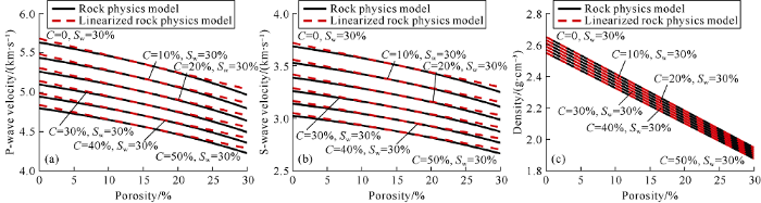
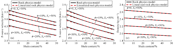
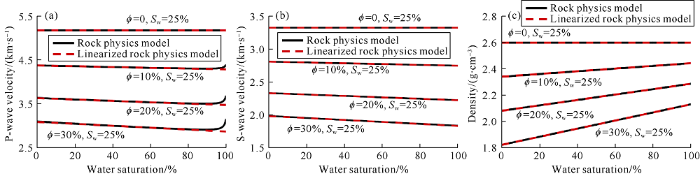
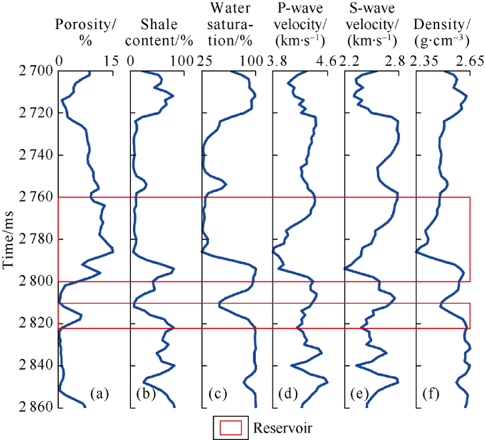
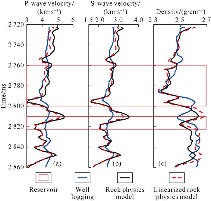
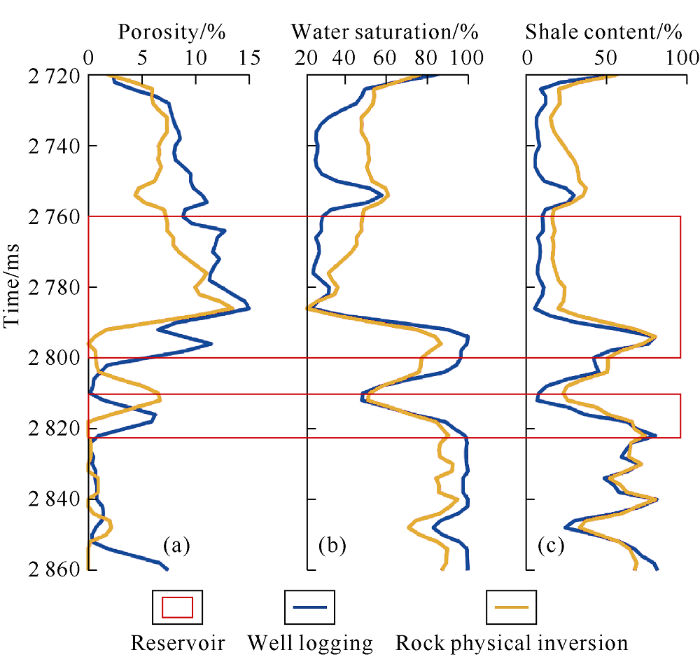

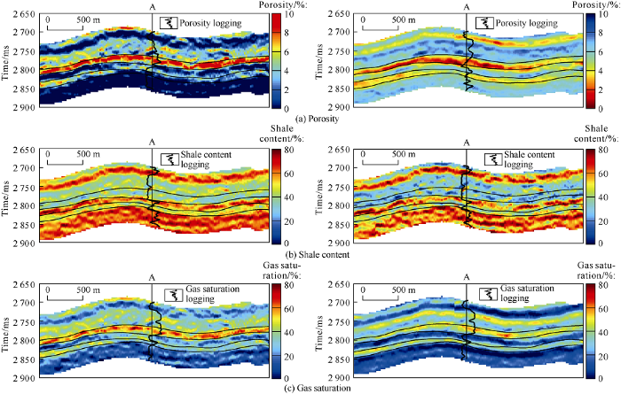
