Productivity simulation of hydraulically fractured wells based on hybrid local grid refinement and embedded discrete fracture model

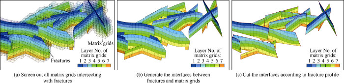
Fig. 1. Grid generation in embedded discrete fracture model (EDFM).

When the fracture size is larger than the matrix grid, the interface between the matrix grid and the fracture is smaller than the fracture, and the fracture is finally divided into multiple fracture slices (Fig. 1c). There are usually many fractures in the model, and each fracture will be divided into a series of slices. All the fracture pieces form a set of grid system, which is called "fracture grid system" composed of unstructured grids that can’t be numbered with (I, J, K).

The methods proposed by Lee et al.^[23,24] and Moinfar et al.^[19,20] are mainly used to calculate the conductivity between matrix grid and fracture slice, between fracture piece and fracture piece. These methods are based on two-point cases. If T represents the conductivity, flow term of any two units (from a to b) can be written as$\lambda T\left( {{\Phi }_{a}}-{{\Phi }_{b}} \right)$. For the flow term within and between fractures, a straight line with unit slope is used for relative permeability.

In the interior of fracture slice, the conductivity is calculated according to the difference format of planar polygon. If two fracture slices are intersected (Fig. 2a), the equivalent conductivity is the harmonic average of the conductivity from the two fracture slices to the intersection line:

(1) $\left\{ \begin{align} & {{T}_{\text{ff}}}={{\left( \frac{1}{{{T}_{\text{f}1}}}+\frac{1}{{{T}_{\text{f2}}}} \right)}^{-1}} \\ & {{T}_{\text{f}1}}=\frac{{{H}_{1}}L}{{{{\bar{d}}}_{\text{f}1}}}{{K}_{\text{f}1}} \\ & {{T}_{\text{f2}}}=\frac{{{H}_{2}}L}{{{{\bar{d}}}_{\text{f}2}}}{{K}_{\text{f2}}} \\ \end{align} \right.$

Fig. 2.

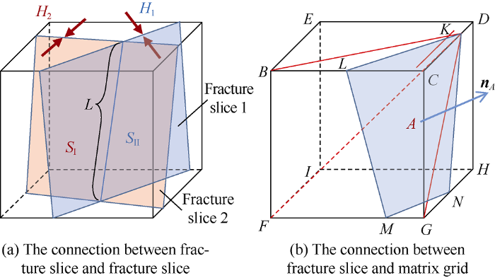
Fig. 2. Schematic diagram of connection between two fracture slices and between fracture slice and matrix grid.

The average distance from all infinitesimals in the fracture slice to the intersection line is:

(2)${{\bar{d}}_{\text{f}}}=\frac{\int_{S}{\left\| \mathbf{d} \right\|\text{d}S}}{S}$

Generally, one fracture passing a intersecting line is divided into two sub- polygons by the intersecting line. If I and II represent the two sub-polygons, then ${{\bar{d}}_{\text{f}}}$can be calculated according to Eq. (3).

(3)${{\bar{d}}_{\text{f}}}=\frac{{{S}_{\text{I}}}{{d}_{\text{I}}}+{{S}_{\text{II}}}{{d}_{\text{II}}}}{{{S}_{\text{I}}}+{{S}_{\text{II}}}}$

Since the fracture slice is embedded in the hexahedral matrix grid, the conductivity between the matrix grid and the fracture slice cannot be calculated by conventional method, and is equal to:

(4)${{T}_{\text{mf}}}=\frac{A}{{\bar{d}}}{{K}_{\text{m}}}$

If the permeability of matrix is tensor, the conductivity is equal to:

(5)${{T}_{\text{mf}}}=\frac{A}{{\bar{d}}}\left( {{\mathbf{n}}_{A}}\cdot {{K}_{\text{m}}}\cdot {{\mathbf{n}}_{A}} \right)$

The distance $\bar{d}$ from matrix grid to fracture slice is the distance between the pressure representative point of matrix and fracture slice. It is equal to the average distance from each infinitesimal of matrix to fracture slice, which can be written as:

(6)$\bar{d}=\frac{\int_{V}{\left\| \mathbf{d} \right\|\text{d}V}}{V}$

In the calculation of $\bar{d}$, Moinfar et al.^[19-20]used numerical integration, that is, a matrix grid is divided into several infinitesimals, to calculate the volume weighted average of$\left\| \mathbf{d} \right\|$. This method has the tricky issue of balancing accuracy and efficiency. In fact, $\bar{d}$is the weighted average of the distance from six pyramids to the fracture slice which can be accurately calculated, to avoid numerical integration. As shown in Fig. 2b, the bottom of each pyramid is a face of the hexahedron, and the vertices of the pyramid are the same points on the fracture slice. For convenience, the first vertex of the fracture slice is taken as the base point (point K in Fig. 2b). The average distance between the hexahedron and the fracture slice KLMN can be expressed as:

(7)$\bar{d}=\frac{{{\left( dV \right)}_{K-BCDE}}+{{\left( dV \right)}_{K-FGHI}}+{{\left( dV \right)}_{K-BFIE}}+{{\left( dV \right)}_{K-CDHG}}+{{\left( dV \right)}_{K-BCGF}}+{{\left( dV \right)}_{K-DEIH}}}{{{V}_{K-BCDE}}+{{V}_{K-FGHI}}+{{V}_{K-BFIE}}+{{V}_{K-CDHG}}+{{V}_{K-BCGF}}+{{V}_{K-DEIH}}}$

In Eq. (7), " K-****" refers to a pyramid with a vertex of K. When the bottom of the pyramid is on the same side of the fracture slice (e.g. K-BFIE), d is equal to the distance between the center of mass of the pyramid and the fracture slice (the center of mass of the pyramid is at 3/4 of the center of the pyramid from the vertex); when the bottom of the pyramid is divided by an edge of the fracture slice (e.g. K-BCGF, BCGF is divided by LM), d is equal to the weighted average of the distance between two pyramids (K-BLMF, K-LCGM) and fracture slice. In Fig. 2b, d and volume of K-BCDE and K-CDHG are both zero, which is related to the selection of vertex K of pyramid. The value of formula (7) is the same as long as K is taken as a vertex of the fracture slice.

1.1.2. Heterogeneous permeability of embedded fractures

The mainstream EDFM simplifies the fracture as a thin slice with uniform permeability, which is not consistent with the actual geologic situation. Thus, it is necessary to consider the heterogeneity of permeability in the fracture. In this study, the lattice data of fracture aperture in the calculation results of fracturing simulation was mapped to the embedded fractures, and the permeability of each fracture piece of embedded fractures was calculated by using the aperture data. When calculating the permeability, it was assumed that the flow in the fractures was flat laminar flow, so the permeability of the fracture conformed to the cubic law. The permeability of any point x of the fracture is equal to${{K}_{0}}\frac{w{{\left( x \right)}^{3}}}{{{w}_{0}}^{3}}$, where$w\left( x \right)$ is the aperture of the fracture at point x, K₀ is the permeability of the fracture root, and${{w}_{0}}$is the aperture of the fracture root. The root of fracture is the point where it is connected with the wellbore, and it is also the position where fracture aperture is maximum. $w\left( x \right)$is obtained by linear interpolation of aperture lattice data. The permeability of a fracture slice (area: Ω) is equal to the harmonic average of the permeability of all points in the fracture slice^[28]:

(8)${{K}_{\Omega }}={{K}_{0}}\Omega {{\left\{ \int\limits_{\Omega }{{{\left[ \frac{w{{\left( x \right)}^{3}}}{{{w}_{0}}^{3}} \right]}^{-1}}\text{d}\Omega } \right\}}^{-1}}$

Formula (8) can be used for numerical integration to calculate the heterogeneous permeability of artificial fracture grids. Fracture slices with permeability equal to zero are regarded as invalid grids, and are eliminated from the simulation.

1.1.3. Local grid refinement near artificial fractures

The advantage of EDFM is that fractures do not affect the shape of matrix grid, but matrix grids too large would lead to sparse grids in and around fractures, making it difficult to describe the complex seepage process near the wellbore and impairing the simulation accuracy. In actual reservoirs, artificial fractures are usually tens of meters to 200 meters in half-length, and the size of matrix grids in geological model can be more than 100 meters. If the geological model was directly used, the half-wing of a fracture would be only discretized into 1-2 fracture slices in the horizontal direction, which would bring great error to the productivity prediction. Therefore, in this study, a coupling method of local grid refinement (LGR) and EDFM was adopted. Firstly, the matrix grids near the wellbore were refined orthogonally, and then the artificial fractures were "embedded" into the matrix grid after densification. As the matrix grids were finer, the fracture pieces formed after the cutting by matrix grids were also finer. In other words, the embedded fracture pieces were refined with the matrix grids, which improved the accuracy of fluid flow calculation in the near wellbore zone and inside the fracture.

The application of LGR and EDFM at the same time makes the process of fracture segmentation very complicated. When dealing with the connection between fractures and matrix grids, the connection between embedded fracture pieces and refined grids should be considered. Besides, when dealing with the connection of fracture pieces inside the fractures, the situation of fractures entering refinement areas from matrix grids and fractures crossing refinement areas should also be considered. Due to the different refinement degrees in different areas, the fractures passing through two refinement areas could have the situation that the adjacent grid boundaries are not aligned (Fig. 3). In this case, the conductivity between the two grids needs special treatment. Suppose that the unit nor-mal vector of the common edge of two grid elements a and b is$n$, and ${{p}_{a}}$,${{p}_{b}}$are vectors from the center of a and b to the midpoint of the common boundary, the length of the common boundary is L_ab, and the fracture aperture is H, then the calculation formula of the conductivity between a and b is:

(9)${{T}_{ab}}=H{{L}_{ab}}{{\left[ \frac{1}{{{{K}_{a}}\left( {{p}_{a}}\cdot n \right)}/{{{\left\| {{p}_{a}} \right\|}^{\text{2}}}}\;}+\frac{1}{{{{K}_{b}}\left( {{p}_{b}}\cdot n \right)}/{{{\left\| {{p}_{b}} \right\|}^{\text{2}}}}\;} \right]}^{-1}}$

Fig. 3.

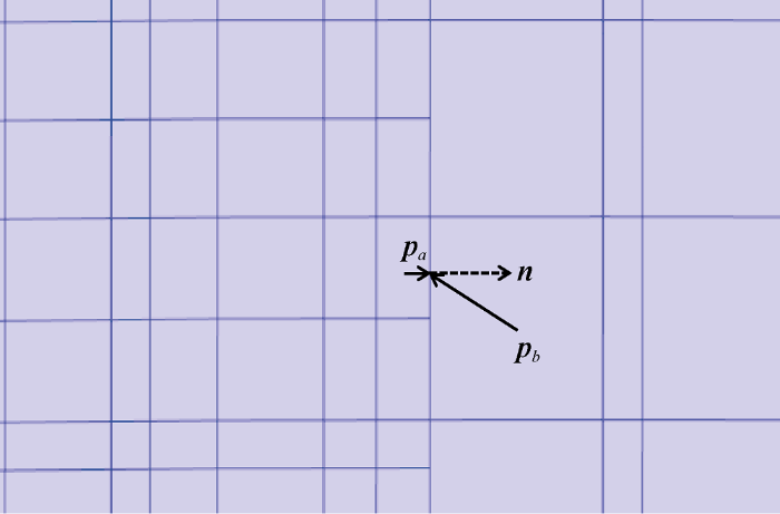
Fig. 3. Diagram of conductivity calculation of misaligned grids.

1.2. Numerical solution

The numerical model of productivity calculation for fractured well based on EDFM includes three groups of control equations: matrix grid, fracture grid and wellbore, forming a set of coupled nonlinear equations. In this study, in order to ensure the convergence speed of solving the coupled equations, the Newton full implicit method was used. When generating Jacobian matrix, it was required to take the derivatives of all equations to all independent variables, and the final Jacobian matrix was a block matrix with the dimension of 3 × 3, which was composed of 7 parts. The three rows of the matrix correspond to control equations of matrix grids, fracture grids and wellbore, respectively. The three columns of the matrix correspond to three groups of independent variables: matrix grids, fracture grids and wellbore (Fig. 4). The letters M, F and W in Fig. 4 represent matrix, fracture and wellbore, respectively. In the naming of the matrix block, the first letter represents equation, the second letter represents variable. For example, "MF" represents derivative matrix of equations of matrix grids to fractures variable (there is source sink term of inflow fracture in matrix equations), and "FW" represents derivative matrix of fracture equations to well variable (there is source sink term of inflow well in fracture equation). This model does not consider the flow of matrix into the wellbore, so there is no “MW” and “WM” matrix.

Fig. 4.

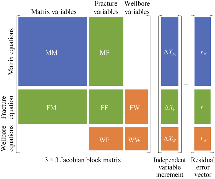
Fig. 4. Linear equations of matrix-fracture-wellbore system.

2. An example of a vertical fractured well in tight reservoir

Well V5X in tight reservoir S of H Oilfield in Iraq is taken as an example. The total reserves of S reservoir account for 25% of the total reserves of H Oilfield, but its production contribution is less than 1%. The S reservoir is poor in petrophysical properties, with an average permeability of 0.6×10^-3 μm² and average porosity of 13%. It belongs to "medium porosity and low permeability" carbonate reservoir.

Well V5X was put into production in August 2014. Matrix acidizing and acid fracturing stimulation measures were taken in the early stage, but the output was low and the effective period was short. The well could not meet the production allocation requirements, and was in the state of intermittent production. In order to produce the S reservoir effectively, the first proppant fracturing pilot test was carried out in this well in December 2016. In the fracturing, 443.5 m³ of fluids and 39.6 m³ of sand in total were injected at the pumping rate of 5.5 m³/min. After fracturing, the well tested an oil production of 217.8 m³/d, which was 9.4 times the production before fracturing. The well has been producing under controlled pressure, had an average production of 81.8 m³/d, and cumulative oil production of about 8.9 × 10⁴ m³ in the three years after fracturing.

According to the actual treatment parameters, the fracturing process was simulated by software FracproPT to obtain the main fracture parameters as shown in Table 1.

Table 1 Main fracture parameters of Well V5X.

Fracture parameter	Value	Fracture parameter	Value
Propped half length	94 m	Depth of fracture bottom	2 765 m
Maximum propped height	65 m	Dynamic aperture	1.2 cm
Depth of fracture top	2 700 m	Conductivity	40 μm²•cm

Based on reservoir engineering analysis, the control range of well V5X is 2000 m × 2000 m. Accordingly, the single well model was cut out from the reservoir model while the attribute data remained the same with the original model. The half- length of the propped fracture was 94 m, and the size of matrix grids was 100 m. In this case, the local grids near the wellbore zone were refined. The fracture growth process in well V5X was simulated by the fracture software to get the initial fracture aperture. The heterogeneous permeability was set for the embedded fracture by the method mentioned above. According to the method proposed in this paper, a single well model with EDFM was built. In the simulation study, the production mode of the well was set as constant oil production of 130.9 m³/d, and the minimum bottom hole pressure was set at 19.3 MPa. Under constant oil production mode, when the bottom hole pressure dropped to the lowest pressure, it was converted to the production mode of constant bottom hole pressure.

2.1. Refinement times of the grids

Theoretically, the denser the matrix grids near the wellbore are, the higher the calculation accuracy will be. But when the grid refinement times reach a certain degree, the increase of calculation accuracy slows down, and the calculation amount of the model increases greatly. Therefore, there is an optimal grid refinement times. Therefore, an EDFM model was established by using fracture parameters obtained from the fracturing simulation software. Productivities of the fractured well V5X without refinement and with the refinement times of 4, 8, 16 and 32 were simulated respectively (Fig. 5). The calculation results of the cumulative oil production were counted. The cumulative oil production at the refinement times of 32 was taken as the base and the relative errors between the cumulative oil production at other refinement times and the base were calculated. The results are shown in Table 2.

Fig. 5.

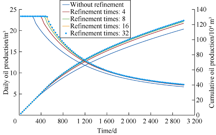
Fig. 5. Changes of simulated production rates and cumulative production of fractured well under different refinement times.

Table 2 Comparison of cumulative oil production calculated at different refinement times.

Refinement times	Cumulative production/ 10⁴ m³	Relative error/%	Refinement times	Cumulative production/ 10⁴ m³	Relative error/%
1	21.112	-5.70	16	22.307	-0.37
4	21.734	-2.90	32	22.389
8	22.127	-1.20

It can be seen from Fig. 5 and Table 2 that the productivity prediction results after grid refinement are quite different from those without refinement. With the increase of refinement times, the productivity of the fractured well shows an overall "increase" trend. This is because when the refinement times are low, the matrix grids near wellbore are larger, and can’t describe the complex seepage process with the presence of artificial fractures. Thus, the simulation results have larger errors. With the increase of refinement times, the increase speed of cumulative oil production gradually decreases. In the no-refinement case, the mesh size of matrix grids is 100 m, which is close to the half-length of the fracture. When the refinement is 16 times of the original grid size, the simulation result of cumulative oil production is almost stable, and the relative error is only -0.37% compared with the refinement of 32 times. This means the refinement of 16 times in near wellbore zone is appropriate, which can not only ensure the calculation accuracy, but also save calculation time. In the actual simulation, it is suggested to set the mesh size of matrix grid to 1/10 of the half-length of hydraulic fractures, so that the calculation accuracy and calculation time can be well balanced.It should be noted that the heterogeneity of fracture permeability distribution will have a great impact on the simulation results. The fracture permeability has a cubic relationship with fracture aperture, and is related to the direction of fracture length. In this case, if the heterogeneity of fracture permeability was not considered and the permeability at the root of fracture was adopted uniformly, the cumulative oil production after 3000 days from simulation would be 11.1% higher than that considering the heterogeneity of permeability under the refinement of 32 times. This is mainly due to the overestimation of overall conductivity of the artificial fracture. Apparently, the simulation considering the permeability heterogeneity of artificial fracture is more consistent with the real situation.

2.2. Case validation

2.2.1. Comparison with DFN model

On the basis of optimization of grid refinement times, EDFM and DFN methods were used to simulate the case. Fig. 6(a) shows the grid generation results of EDFM. DFN adopted vertical bisection grids (PEBI), and Fig. 6 (b) shows the grid generation results of DFN containing 201 312 cells. Fig. 7 shows the simulation results by the two models. Fig. 8 shows the pressure distributions 1000 days after fracturing by the two methods. It can be seen that the productivity and pressure distribution simulated by EDFM are basically consistent with those simulated by DFN.

Fig. 6.

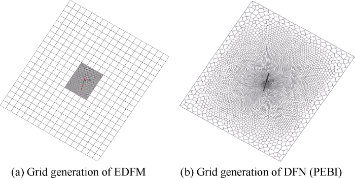
Fig. 6. Schematic diagram of grid generation of EDFM and DFN.

Fig. 7.

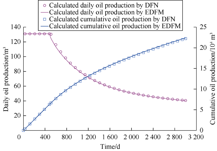
Fig. 7. Comparison of oil production simulated by EDFM and DFN.

Fig. 8.

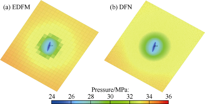
Fig. 8. Pressure distribution 1 000 days after fracturing simulated by EDFM and DFN models.

Table 3 shows simulation parameters of EDFM and DFN models. EDFM can not only ensure the accuracy of simulation, but also reduce the number of grids, save calculation cost and improve simulation efficiency. It has great technical advantages in actual reservoir simulation.

Table 3 Comparison of simulation parameters of EDFM and DFN models.

Simulation method	Total grids	Fracture grids	Total time steps	Truncation time steps	Total Newton iteration steps	CPU time consumed/s
EDFM	52 501	805	107	1	299	160
DFN	201 312	5 772	108	2	425	1 229

2.2.2. Validation with actual production data

History matching of two stages (before and after fracturing) of Well V5X was carried out. Before fracturing (August 2014 to December 2016), the production history was matched based on the actual bottom-hole pressure. On the basis of history matching, the restart file was established. The fracture parameters in Table 1 were used to add fractures in EDFM. After fracturing (December 2016 to November 2018), the production history was also matched (Fig. 9). It can be seen that the daily oil production and bottom-hole flow pressure calculated by the model are in good agreement with the actual production data, proving that the model is correct and reliable.

Fig. 9.

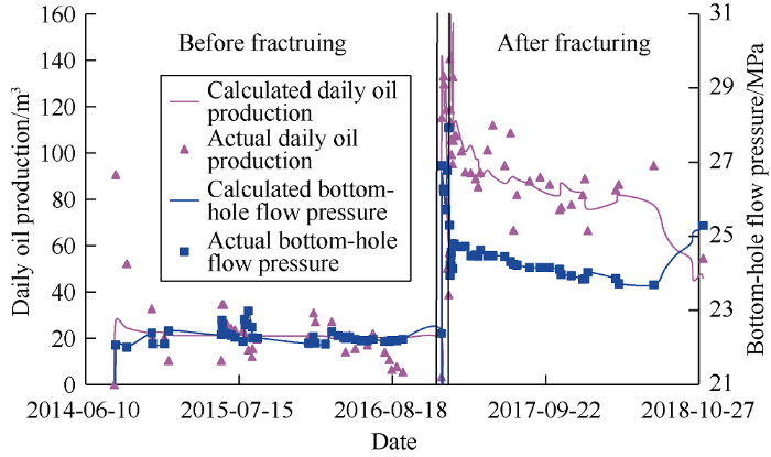
Fig. 9. History matching results of Well v5x.

3. Parameters optimization of multi-stage fracturing for a horizontal well

After the preliminary success of the pilot well V5X, it was planned to carry out pilot test of the first multi-stage fracturing of horizontal well in the same formation. “LGR-EDFM coupling method” was used to optimize the fracture parameters of multi-stage fracturing for horizontal well and guide the fracturing process design. EDFM has two advantages in practical application: (1) When modifying the fracture size and stage spacing, it doesn’t need to re-divide the grids. (2) The matrix grids remain unchanged so that the simulation cases are more comparable.

3.1. Establishment of model

The fracture parameters were obtained from fracturing simulation and input into the reservoir numerical simulation model. Artificial fractures were modeled by the EDFM method and matrix grids near the wellbore were refined (Fig. 10). The production mode of the horizontal well was set as constant oil production of 245.5 m³/d, and the minimum bottom-hole pressure was set at 19.3 MPa. When the bottom-hole pressure drops to the lowest value, the well was converted to the production mode under constant bottom-hole pressure.

Fig. 10.

Fig. 10. “Coupled LGR-EDFM model” for simulating horizontal well multi-stage fracturing.

3.2. Optimization of stimulation parameters

The horizontal well productivities at horizontal section lengths of 600, 800, 1000 m, fracturing stages of 6, 8, 10, fracture half-lengths of 110, 130, 150 m, and fracture conductivity of 20, 40, 60 μm²•cm were simulated. According to the principle of orthogonal design, 9 cases were designed (Table 4) and simulated.

Table 4 Orthogonal design cases.

No.	Length of horizontal section/m	Stages	Half-length of fracture/m	Fracture conductivity/(μm²•cm)
1	600	6	110	20
2	600	8	130	40
3	600	10	150	60
4	800	6	130	60
5	800	8	150	20
6	800	10	110	40
7	1 000	6	150	40
8	1 000	8	110	60
9	1 000	10	130	20

The simulation results of cumulative oil production of the horizontal well in the 9 cases are shown in Fig. 11. It can be seen from the figure that case 7 has the highest cumulative oil production, and case 1 has the lowest. The cumulative oil production in descending order of the cases are case 7, case 8, case 9, case 4, case 6, case 5, case 3, case 2 and case 1. The productivity of horizontal well is most sensitive to the length of horizontal section, the cumulative oil production of the case with the horizontal section length of 1000 m is greater than the cases with 800 m and 600 m. The case 7 has the optimal design parameters and highest productivity.

Fig. 11.

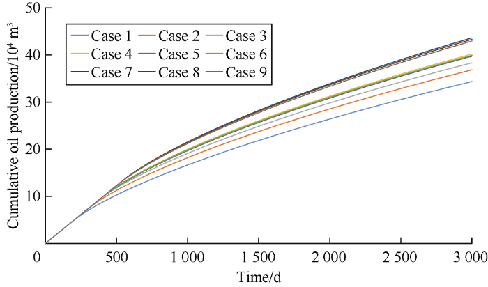
Fig. 11. Comparison of cumulative oil production of the horizontal well in different cases.

4. Conclusions

In view of the incompatibility of EDFM in corner grid system including the low accuracy in the near-wellbore zone, and the non-uniformity of the conductivity in the fractures without considering the heterogenous conductivity, a new EDFM in corner grid system is designed, which can realize the efficient calculation of the conductivity of the embedded fractures and matrix grids. The permeability of each fracture piece of embedded fractures is calculated by using the lattice data of artificial fracture aperture. On this basis, a coupling method of local grid refinement and embedded discrete fracture model is proposed to predict the productivity of the fractured well.

The validity of the method has been verified by comparing its calculation results with those from DFN method and fitting the actual production data of the first hydraulically fractured well in the Middle East. Combined with orthogonal design, this method can be used to optimize the parameters of multi-stage fracturing for horizontal wells. The method proposed in this paper has theoretical significance and strong practicability for improving the adaptability of EDFM and productivity prediction accuracy, and enables the coupling solution of fracture simulation and productivity numerical simulation at reservoir scale.

Nomenclature

a, b—grid unit;

A—fracture area in the matrix grid or unit control volume, m²;

d—height of the pyramid, m;

${{\bar{d}}_{{}}}$—average distance from each infinitesimal of the matrix to the polygon, m;

d—vertical vector from planar infinitesimal to the intersection line, m;

${{\bar{d}}_{\text{f}}}$—average distance from all the infinitesimals in fracture slice to the intersection line, m;

${{\bar{d}}_{\text{f1}}}$, ${{\bar{d}}_{\text{f2}}}$—average distance from all the infinitesimals in fracture slice 1 and 2 to the intersection line, m;

${{d}_{\text{I}}}$, ${{d}_{\text{II}}}$—distance from the center of gravity of two sub polygons to the intersection line, m;

H—fracture aperture, m;

H₁, H₂—aperture of fracture slice 1 and 2, m;

I, J, K—grid number index symbol;

K₀—permeability at the fracture root, 10^-3 μm²;

K_a, K_b—permeability of grid units a and b in matrix, 10^-3 μm²;

K_f1, K_f2—permeability of fracture slice 1 and 2, 10^-3 μm²;

K_m—matrix permeability, 10^-3 μm²;

${{K}_{\text{m}}}$—permeability tensor of matrix, 10^-3 μm²;

${{K}_{\Omega }}$—permeability of polygon with an area of Ω in the fracture slice, 10^-3 μm²;

L_ab—length of the intersection line between two fractures, m;

n—unit normal vector of the common edge of two grid elements a and b;

n_A—external normal vector of fracture slice element A;

p_a, p_b—vectors from the center of a and b to the midpoint of the common boundary;

r—residual error;

S—area of fracture slice, m²;

${{S}_{\text{I}}}$, ${{S}_{\text{II}}}$—area of the sub-polygons, m²;

T—conductivity, 10^-3 μm²•m;

T_ab—conductivity between grid elements a and b, 10^-3 μm²•m;

T_f1, T_f2—conductivity of fracture slice 1 and 2 to the intersection line, 10^-3 μm²•m;

T_ff—harmonic average conductivity, 10^-3 μm²•m;

T_mf—conductivity between matrix grid and fracture slice, 10^-3 μm²•m;

V—volume of matrix grids, m³;

w₀—aperture of fracture root, m;

w(x)—fracture aperture at point x, m;

x—joint coordinates inside the fracture, m;

ΔX—increment of independent variable;

$\lambda $—fluid mobility, 10^-3 μm²/(mPa•s);

${{\Phi }_{a}}$, ${{\Phi }_{b}}$—pressure potential or head of grid elements a and b, MPa;

Ω—area of fracture slice, m².

Subscript:

F—fracture;

M—matrix;

W—wellbore.

Reference

By original order

By published year

By cited within times

By Impact factor

[1]

JIA

Chengzao

, ZHENG

Min

, ZHANG

Yongfeng

Unconventional hydrocarbon resources in China and the prospect of exploration and development

Petroleum Exploration and Development, 2012,39(2):129-136.

[2]

CHEN

Qilin

, DENG

Yilin

, WEI

Jun

, et al.

Types, distribution and play targets of Lower Cretaceous tight oil in Jiuquan Basin, NW China

Petroleum Exploration and Development, 2018,45(2):212-222.

[3]

NELSON P

Pore-throat sizes in sandstones, tight sandstones, and shales

AAPG Bulletin, 2009,93(3):329-340.

DOI:10.1038/srep36919 URL PMID:27830731 [Cited within: 1]

Understanding the pore networks of unconventional tight reservoirs such as tight sandstones and shales is crucial for extracting oil/gas from such reservoirs. Mercury injection capillary pressure (MICP) and N₂ gas adsorption (N₂GA) are performed to evaluate pore structure of Chang-7 tight sandstone. Thin section observation, scanning electron microscope, grain size analysis, mineral composition analysis, and porosity measurement are applied to investigate geological control factors of pore structure. Grain size is positively correlated with detrital mineral content and grain size standard deviation while negatively related to clay content. Detrital mineral content and grain size are positively correlated with porosity, pore throat radius and withdrawal efficiency and negatively related to capillary pressure and pore-to-throat size ratio; while interstitial material is negatively correlated with above mentioned factors. Well sorted sediments with high debris usually possess strong compaction resistance to preserve original pores. Although many inter-crystalline pores are produced in clay minerals, this type of pores is not the most important contributor to porosity. Besides this, pore shape determined by N₂GA hysteresis loop is consistent with SEM observation on clay inter-crystalline pores while BJH pore volume is positively related with clay content, suggesting N₂GA is suitable for describing clay inter-crystalline pores in tight sandstones.

[4]

ZHANG

Fudong

, LI

Jun

, WEI

Guoqi

, et al.

Formation mechanism of tight sandstone gas in areas of low hydrocarbon generation intensity: A case study of the Upper Paleozoic in North Tianhuan depression in Ordos Basin, NW China

Petroleum Exploration and Development, 2018,45(1):73-81.

[5]

Suyun

, ZHU

Rukai

, WU

Songtao

, et al.

Profitable exploration and development of continental tight oil in China

Petroleum Exploration and Development, 2018,45(4):737-748.

[6]

JIANG

Ruizhong

, XU

Jianchun

, FU

Jianbin

Multistage fractured horizontal well numerical simulation and application for tight oil reservoir

Journal of Southwest Petroleum University (Natural Science Edition), 2015,37(3):45-52.

[Cited within: 2]

[7]

FAN

Jianming

, YANG

Ziqing

, LI

Weibing

, et al.

Assessment of fracturing treatment of horizontal wells using SRV technique for Chang-7 tight oil reservoir in Ordos Basin

Journal of China University of Petroleum (Natural Science Edition), 2015,39(4):103-110.

[8]

WANG

Wendong

, SU

Yuliang

, MU

Lijun

, et al.

Influencing factors of simulated reservoir volume of vertical wells in tight oil reservoirs

Journal of China University of Petroleum (Natural Science Edition), 2013,37(3):93-97.

[9]

JIANG

Longyan

, XUN

Xiaoquan

, WANG

Nan

, et al.

Non-steady state productivity evaluation model of volume fracturing for vertical well in tight oil reservoir

Fault-Block Oil & Gas Field, 2015,22(1):82-84.

[10]

SHI

Xiaodong

Productivity forecast of vertical well with multi-layer network fracturing in tight oil reservoir

Special Oil and Gas Reservoirs, 2017,24(1):124-127.

[11]

BARENBLATT G

, ZHELTOV I

, KOCHINA I

Basic concepts in the theory of seepage of homogeneous liquids in fissured rocks [strata]

Journal of Applied Mathematics and Mechanics, 1960,24(5):1286-1303.

DOI:10.1016/0021-8928(60)90107-6 URL [Cited within: 1]

[12]

WARREN J

, ROOT P

The behavior of naturally fractured reservoirs

Society of Petroleum Engineering Journal, 1963,3(3):245-255.

DOI:10.1038/s41598-018-30097-2 URL PMID:30072702 [Cited within: 1]

In the past few decades, scholars have made great breakthroughs in the study of well test analysis of carbonate rock. The previous studies are based on horizontal wells, straight wells, fractured wells, and inclined wells. With the development of fracturing technology, acid fracturing technology is considered to be the most effective measure to develop carbonate reservoirs. As the carbonate rock is easily dissolved in carbonic acid, multi-branched fractures will be produced near a vertical well. This article presented a semi-analytical model for multi-branched fractures in naturally fractured-vuggy reservoirs for the first time, which laid a theoretical foundation for solving well test analysis for finite conductivity multi-branched fractures. The model can quantify the wellbore flow pressure and applied to obtain more parameters reflecting comprehensive flow characteristics through using history matching procedure. The results were compared with numerical simulation and the existing analytical solutions of a single fracture model. Then in this paper, flow characteristics are recognized and there are five flow regimes found in the type curves, e.g. bi-linear flow region, linear flow region, inter-porosity flow region between vugs and fractures, inter-porosity region between matrix and fractures, and radial flow region. Finally, the influence factors analysis shows fracture number will mainly affect flow behavior of bi-linear flow and linear flow. The angle analysis showed that as the fractures were closer, their interaction became stronger. The conductivity would seriously affect the flow behavior in the early time. Linear flow cannot be observed when the conductivity is less than 1 and bi-linear flow cannot be observed when the conductivity is more than 20. And the effect of fracture length on flow behavior occurs in the early time. Bi-linear flow and linear flow characteristics cannot be observed when the fracture length is reduced.

[13]

THOMAS L

, DIXON T

, PIERSON R

Fractured reservoir simulation

Society of Petroleum Engineers Journal, 1983,23(1):42-54.

DOI:10.2118/9305-PA URL [Cited within: 1]

[14]

GHORAYEB

, FIROOZABADI

Numerical study of natural convection and diffusion in fractured porous media

Society of Petroleum Engineers Journal, 2000,5(1):12-20.

[15]

LYU

Xinrui

, YAO

Jun

, HUANG

Zhaoqin

, et al.

Study on discrete fracture model two-phase flow simulation based on finite volume method

Journal of Southwest Petroleum University (Natural Science Edition), 2012,34(6):123-130.

[16]

YAO

Jun

, WANG

Zisheng

, ZHANG

Yun

, et al.

Numerical simulation method of discrete fracture network for naturally fractured reservoirs

Acta Petrolei Sinica, 2010,31(2):284-288.

[17]

YANG

Jian

, LYU

Xinrui

, LI

Jianglong

, et al.

Study on discrete fracture network random generation and numerical simulation of fractured reservoirs

Petroleum Geology and Recovery Efficiency, 2011,18(6):74-77.

[18]

ZHANG

Qingfu

, HUANG

Zhaoqin

, YAO

Jun

, et al.

Multiscale embedded discrete fracture modeling method

Chinese Journal of Computational Mechanics, 2018,35(4):507-513.

[19]

MOINFAR

, VARAVEI

, SEPEHRNOORI

, et al.

Development of a coupled dual continuum and discrete fracture model for the simulation of unconventional reservoirs

SPE 163647-MS, 2013.

[Cited within: 5]

[20]

MOINFAR

, VARAVEI

, SEPEHRNOORI

, et al.

Development of an efficient embedded discrete fracture model for 3D compositional reservoir simulation in fractured reservoirs

Society of Petroleum Engineers Journal, 2014,19(2):289-303.

DOI:10.2118/7057-PA URL [Cited within: 5]

[21]

, ZHANG D

A multi-continuum multiple flow mechanism simulator for unconventional oil and gas recovery

Journal of Natural Gas Science & Engineering, 2015,26:652-669.