


Introduction
Most of the conventional prediction methods of oil and gas production in use today require a comprehensive description of the reservoir and fluid properties of the field. This process is not only time-consuming but also requires an intensive effort to understand and analyze the field under study[1]. In addition, the accuracy of the prediction results is mainly dependent on the input data of the models, including geological data, petrophysical data and the reservoir characteristic parameters etc.[2]. However, due to the anisotropy and heterogeneity of the reservoir, data acquisition and rock and fluid characterization are challenging[3]. Furthermore, every step of reservoir simulation involves many uncertainties, ranging from uncertainties in the reservoir input data to uncertainties in laboratory studies, which will influence the prediction of reservoir production performance significantly. Traditionally, reservoir engineers use history matching and the concept of material balance to validate model with hard data, yet the level of uncertainties remain high and may influence the predicted fluid production[4,5]. Hence, machine learning techniques have drawn attention in the oil and gas industry, especially in quick evaluation and production prediction[6]. In recent years, some researchers used machine learning to infer the injector/producer relationship of waterflooding reservoirs by taking the injection rate and production rate as input and output respectively[7,8].
One of the main challenges in the oil and gas industry is the management of data and information. Overwhelmed by a large amount of data, engineers sometimes overlook the useful information that would otherwise improve understanding of the reservoir[9]. Hence, Petroleum Data Analysis (PDA) has drawn more and more attention. PDA makes use of data collected in the oil and gas industry to analyze, simulate and optimize production operations[10]. Big Data Analytics is a branch of data science which involves data mining, artificial intelligence, machine learning, and pattern recognition[11]. Machine learning is defined as the investigation on the ability of the computer to learn based on data[12]. It is used to extract prediction models from data. It can be categorized into two main groups, supervised and unsupervised learning. Supervised learning can learn by classifying or labeling the data. The supervised learning algorithm analyzes the trained data and generates a model that can predict new examples from the same type of feature vectors[13]. Unlike supervised learning which labels and maps input and output data, unsupervised learning doesn’t label all of the input data[14]. ANN is one of the machine learning methods most commonly used in the oil and gas industry[15]. Artificial Neural Network (ANN) is a form of mathematical architecture, inspired by biological neural networks and is used for the approximation of function that can depend on a large number of inputs. ANN comes from its skeletal structure in which the input attributes are chosen to optimize the objective function with multiple hidden layers. In recent years, this approach has been adopted in predicting oil production based on geological parameters such as porosity, permeability and water saturation. But as the relationships between the parameters are complex, the prediction process is time-consuming and expensive[16]. ANN has been used in other aspects of oil and gas industry[17,18,19,20,21]. But the application of ANN does not aim to replace the conventional simulators and workflow, but to serve as a complementary tool for the extraction of additional information from the field data[22].
In this paper, an artificial neural network is proposed for modeling oil, gas and water production rates as a function of measured pressure, injection and production data. The production prediction model for waterflooding reservoir is built by training the neural network architecture using features that are uniquely designed to provide better performance. The feature extraction starts from an initial set of measured data and builds derived values (features) intended to be informative and non-redundant, to facilitate the subsequent learning and generalization steps. The feature extraction technique employed in this work is based on physics of fluid flow and a random combination of measurements. Several features are designed, and through a brute force approach, features that do not significantly contribute to the performance of the model are excluded in the final version of the model. The model proposed in this paper is described in detail below and some cases are analyzed with it.
1. Methodology
In neural network, the neural information is stored in the form of weights and bias. The input term with higher weight has a greater effect in the model[23]. In the classical machine learning method, a set of dataset is divided into three subsets, namely, training, validation, and testing data subsets[24]. The training subset is used for computing the gradient and updating the network weights and biases. The error on the validation subset is monitored during the training process. The error of validation subset normally decreases during the initial phase of training, as does the error of training subset. However, when the network begins to over fit the data, the error of the validation subset typically begins to rise. The network weights and biases at the minimum of the validation subset error are kept. The test subset is used to evaluate the trained and validated model. The test subset error is not used during training, but it is used to compare different models. The test subset error throughout the training process can be plotted. If the error of the test subset reaches a minimum at a significantly different iteration number than the validation subset error with the minimum value, the division of the data set may be not reasonable. In this work, 14 years’ production data of a real reservoir in a Malay basin was used to train, validate and test with artificial neural network. The data was separated into 4 parts, 80% for training, 5% for validation, 5% for testing and another 10% for a blind test of the model. Fig. 1 shows the proposed workflow for simulating the production rate of a water flooded reservoir using artificial neural network.
Fig. 1.
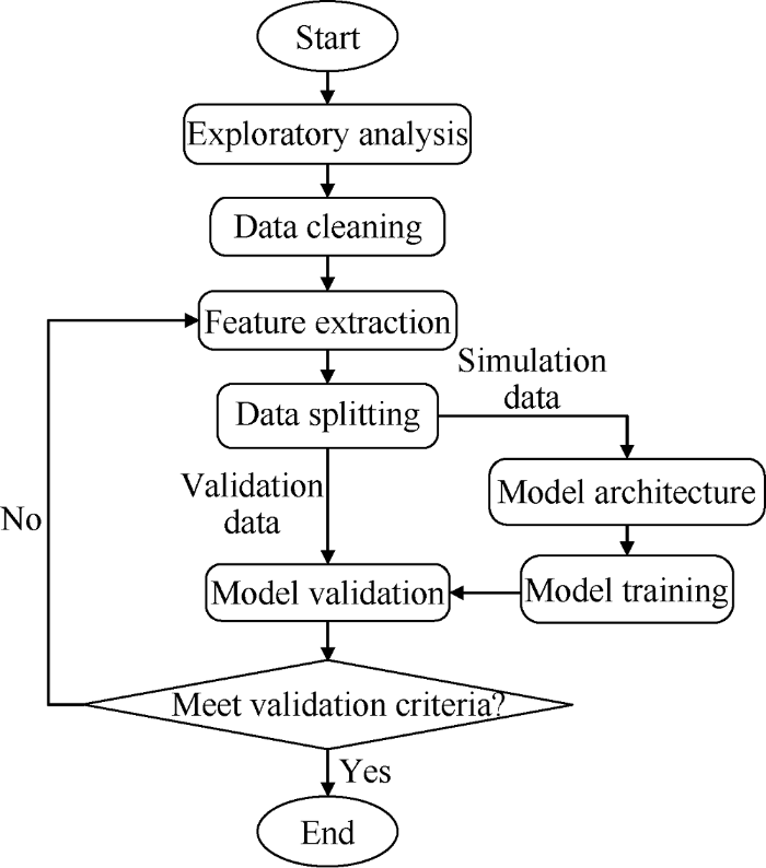
Fig. 1.
Proposed workflow for simulating fluid production rate of a waterflooding reservoir.
1.1. Exploratory analysis
In the exploratory analysis, the dataset is gathered and analyzed. The major source of data is retrieved from Pi-ProcessBook which captures the real-time data sent by the transmitter at the producer and injector. These data are analyzed by using the Pi-ProcessBook and the normal distribution histograms of several features are extracted. Potential outliers and measurement errors are identified from the distribution diagram. In statistics, outliers are data points that don’t belong to a certain population, which are far away from other values. An outlier is an observation value that diverges from other well-structured data. If a data distribution is approximately normal, then about 68% of the data values lie within one standard deviation with the mean and about 95% are within two standard deviations, and about 99.7% lie within three standard deviations. Therefore, outliers are detected by using what is known as the 3σ rule, in which any data that is three or more than three standard deviations away from the mean is considered an outlier.
1.2. Data cleaning
Data cleaning includes finding errors in the datasets and removing or modifying the noise data from the datasets. This process requires understanding of datasets, for one example, understanding the relationship between the injection pressure and flow rate of the injector. This relationship is then used to estimate the injection rate when the flow rate meter is shut down, so the inaccurate data can be then removed. For another example, the offshore daily production report is studied to determine the major events and downtime of the production facilities. In this study, the daily production and water injection data were re-allocated and fine-tuned by cross-checking with different sources of data. Moreover, outlier data points were removed and replaced by using window-based detection method in which the data is divided into fixed size window and then outliers were detected and replaced.
1.3. Feature extraction and expansion
Feature extraction and expansion is the process of using existing datasets to create new input features that make machine learning work and improve its performance. López- Iñesta E et al.[25] proposed and implemented the idea of combining feature extraction and expansion to improve the performance of machine learning. In machine learning, feature extraction refers to the transformation or combination of input data into features. By applying this method, the outcome of machine learning can be improved. In this study, we used features extracted based on fluid physics and random combination of measured data to improve the results of the model. For example, the relationships between the water injection manifold pressure versus the injection pressure of water injector, tubing head pressure, and temperature of oil producer versus the gas lift rate were used. Each term within a feature can be made to have a physical meaning that describes the relationship. Compared with using flow rate and time as separate entities, a combination of the flow rate and time extracted based on the physics of fluid flow and sometimes a random combination may result in better prediction ability of a proposed model. The terms in features from random combinations do not necessarily have a physical meaning. In addition, new features can be obtained by multiplying or dividing of existing ones.
1.4. Optimization algorithm selection
In this project, 3 algorithms, Levenberg-Marquardt, Scaled Conjugate Gradient and Bayesian Regularization, were tested during the training phase. Levenberg-Marquardt Algorithm (LMA) is used to solve non-linear least square problems especially in the least square curve fitting. Many studies have been carried out on using LMA to train Neural Network architecture[26,27,28]. Shi Xiancheng et al.[26] found that a major limitation of LMA was that it obtained a local minimum by only interpolating between the Gauss-Newton algorithm (GNA) and the method of gradient descent. Hence, the accuracy of the model will be affected when there is a large number of training samples and node weights. Scaled conjugate gradient method takes less memory and shorter computation time. It shows better performance in the system of linear equations, but may cause overfitting in the system with many input features[29]. Hence it is not suitable for the training of water flooding reservoir datasets. Bayesian regularization algorithm is found suitable for this project since it adopts the regularization method able to prevent overfitting. Although it takes more time but can result in good generalization of noisy datasets[14]. Bayesian regularization updates the weights and bias of a neural network architecture by minimizing a combination of squared error and weight. Once the minimization is completed, it then determines the correct combination to produce a network that generalizes well.
1.5. Model training
In this study, 90% of the data was used to train, validate and test a model and the remaining 10% was used for blind testing. That is to say 90% of the data was used to train a model architecture and monitor the training process to identify when to stop the training of the model, and then the remaining data was used to blindly test the trained model. In machine learning, the data used in the training step cannot be reused for testing[30].
1.6. Model evaluation
Several performance evaluation indexes were adopted by researchers before[24, 31-32]. In this project, the model was evaluated by using mean square error (MSE), R-square value (R2), and whiteness test[33]. Mean square error is the average square difference between the output and target. The R2 value measures the correlation between the output and target. A model that results in low MSE and R2 value closer to 1 during the testing phase is considered fit. These two indexes are able to indicate whether the model has extracted all the information or needs further tuning. The whiteness test works out the distribution of errors by plotting a histogram. For a good model, the error histogram should indicate a mean value of zero and some variance. In addition, the cross-plot analysis can be used as a graphical and visual method to compare the simulated and actual data. An example of a crossplot is presented in Fig. 2. The plot of these two datasets is compared with a 45° straight line. If the plot of simulated output vs. validation data is above the 45° line, then apparently, the model underestimates the validation data, otherwise, the model overestimates the validation data. In an ideal situation where the model perfectly represents the system, the cross-plot of simulated output and validation data will coincide with the 45° line.
Fig. 2.
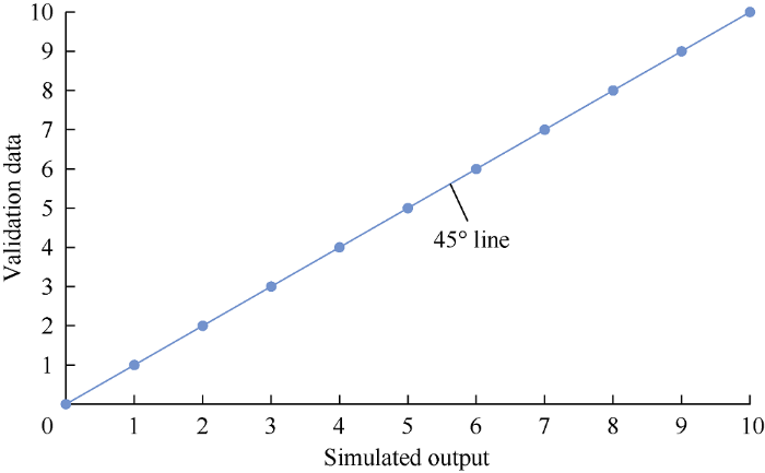
Fig. 2.
Example of a crossplot of simulated output vs. validation data.
2. Case study
2.1. Description of the reservoir and dataset
The data obtained from a reservoir located in Malay basin was used to evaluate the performance of the developed algorithm, and the detail was kept to a minimum due to confidentiality. The reservoir is a saturated reservoir with a small to medium gas cap and a moderate to strong aquifer and is supplementing energy by water injection after 7 years of primary recovery. The PVT properties presented in Fig. 3 shows that the bubble point of the reservoir fluid is approximately 20.68 MPa.
Fig. 3.
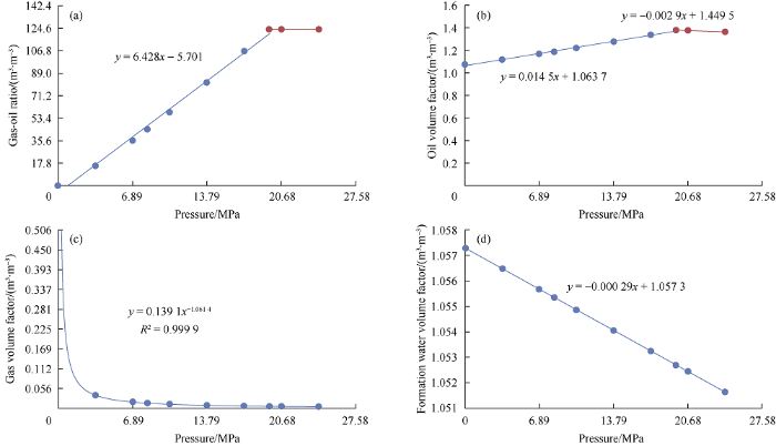
Fig. 3.
PVT properties of the reservoir fluid.
The reservoir was produced by gas cap and aquifer drive from July 1997 to July 2004. The fluid production profile of this period is shown in Fig. 4. From 2004 to 2014, it was produced by water flooding. Oil production rate, gas production rate, water production rate and water injection rate curves of this period are shown in Figs. 5-7, respectively. The data is noisy in such a way that the system cannot understand and interpret correctly. Noise is an unavoidable problem, which affects the data collection and data preparation in machine learning applications. The noise sources from measurement tools.
Fig. 4.
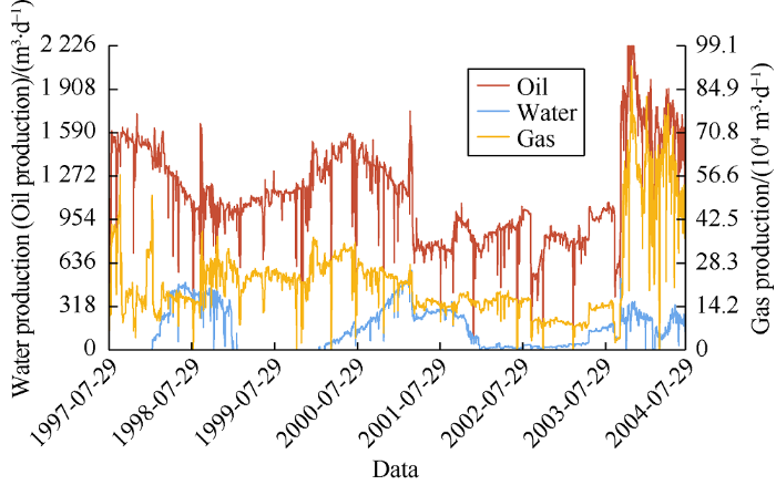
Fig. 4.
Oil, gas and water production before water injection.
Fig. 5.
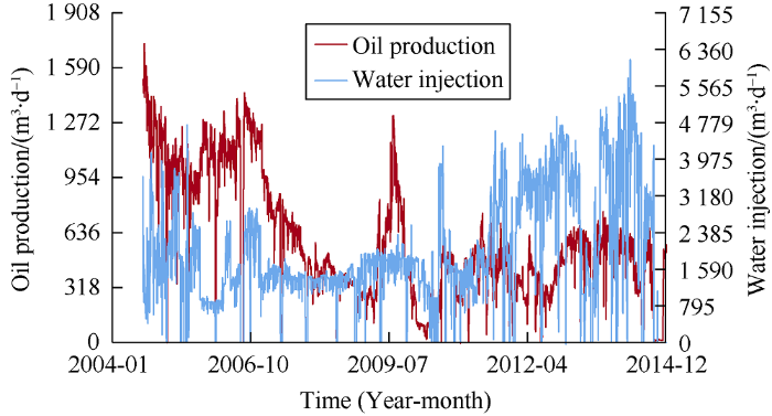
Fig. 5.
Oil production rate of the reservoir after the start of water injection.
Fig. 6.
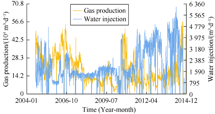
Fig. 6.
Gas production rate of the reservoir after the start of water injection.
Fig. 7.
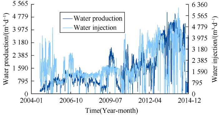
Fig. 7.
Water production rate of the reservoir after the start of water injection.
2.2. Design of input and output data
In order to get more information on the relationship between the water injector and oil producer, a feature extraction technique based on fluid flow physics has been developed. In other words, more features are included to improve the performance of the model. These features are based on combination of the physics of fluid flow in porous media and a simple trial and error combination of terms until a desired goodness of fit between the validation data and simulated output is obtained. Table 1 shows the input and output terms used in this study. Table 2 presents 7 features (No. 1-7) extracted based on physics and random combinations of existing input terms. These features were put to test on the basis of the validation performance of the identified model. Only Features 1, 2 and 5 were used for modeling oil, gas and water flow rates. The time delayed flowrate features are also included in Table 2 (No. 8-13).
Table 1 Input and output terms for modeling oil, gas and water production rates.
| Input | Output | ||
|---|---|---|---|
| Name | Symbol | Name | Symbol |
| Tubing head pressure (producer) | THP | Oil production rate | OPR |
| Tubing heat temperature (producer) | THT | Gas production rate | GPR |
| Gas lift rate (producer) | GLR | Water production rate | WPR |
| Casing pressure (producer) | CP | ||
| Production manifold pressure | PMP | ||
| Water injection rate | WIR | ||
| Water injection manifold pressure | WIMP | ||
| Water injection pressure | WIP | ||
Table 2 Features extracted based on available input and output terms.
| Feature | Form | Physical meaning |
|---|---|---|
| 1 | WIMP(k-1)- WIP(k-1) | One time step delayed pressure difference along the wellbore |
| 2 | THT-GLR | Random combination |
| 3 | WIMP-WIP | The pressure difference along the injection wellbore |
| 4 | WIP/WIMP | The pressure ratio of bottomhole and surface |
| 5 | THP/GLR | Related to gas lifting required to bring fluid to surface |
| 6 | CP-PMP | Pressure loss due to friction and hydrostatic column |
| 7 | (CP-PMP)THT | Random combination |
| 8 | OPR(k-1) | One time step delayed oil flow rate |
| 9 | OPR(k-2) | Two time step delayed oil flow rate |
| 10 | GPR(k-1) | One time step delayed gas flow rate |
| 11 | GPR(k-2) | Two time step delayed gas flow rate |
| 12 | WPR(k-1) | One time step delayed water flow rate |
| 13 | WPR(k-2) | Two time step delayed water flow rate |
Note: k is the No. of the present time step
2.3. Selection of model architecture
Fig. 8 shows a simple architecture of neural network which consists of a single hidden layer, an input layer and an output layer. The number of input parameters and the number of hidden neurons of the ANN model have significant impacts on the final prediction outcome of the model. However, there is limited research on the optimum architecture of the ANN Model. Hence, in this project, different numbers of hidden neurons were set in the architecture of the ANN model, and the optimum architecture of the model was determined based on the results of training and validation performance. During the selection of the number of hidden neurons, it is very important not to have too many parameters to avoid overfitting. Overfitting of a model will result in failure during prediction because overfitted models extract some of the residual variation. Hence, to avoid overfitting, the number of hidden layers are kept to a minimum as much as possible. A series of trials on the training and validation of the dataset was performed to work out the optimum architecture of the model.
Fig. 8.
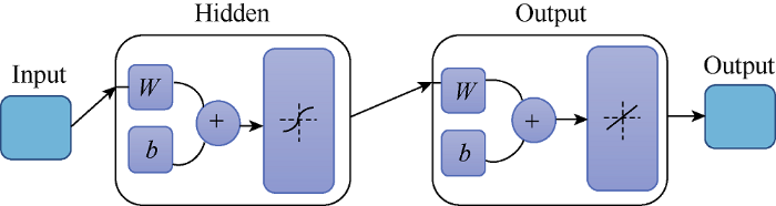
Fig. 8.
Simple architecture of a neural network.
In cases where the data is erratic and required more advanced neural network modeling, a more complex architecture can be considered. Examples of complex architectures commonly used are presented in Figs. 9-11.
Fig. 9.
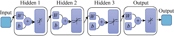
Fig. 9.
Feedforward neural network architecture with three hidden layer.
Fig. 10.
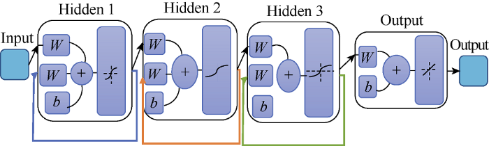
Fig. 10.
Layer-recurrent neural network architecture.
Fig. 11.
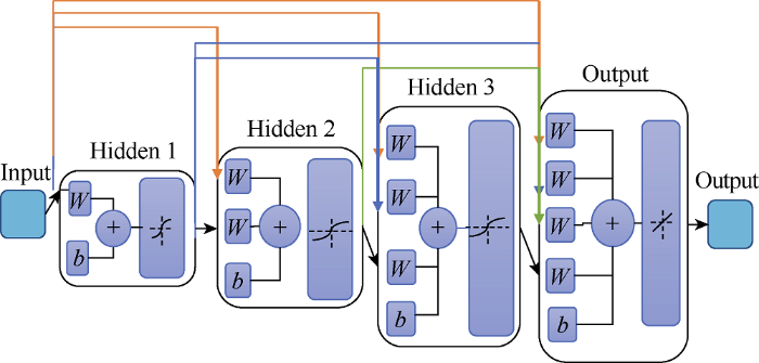
Fig. 11.
Cascade-forward neural network architecture.
2.4. Model training
Based on the results of this study, the Bayesian regularization algorithm is found to be the most suitable learning algo-rithm for training model. The comparison was made based on the R2 exhibited during validation. The training step stopped when the validation error started to increase for six iterations. Bayesian regularization algorithm can generalize noisy datasets and at the same time prevent overfitting[15]. Overfitting is confirmed when R2 for training dataset is higher than that for the testing dataset. The workflow of the Bayesian regularization algorithm is shown in reference [34].
2.5. Model evaluation and production prediction
The predicted data by the model and field measured data were compared, the MSE and R2 of the model predicted data were calculated, and the error distribution histogram was plotted. The model is considered validated when the final mean square error (MSE) and the mean of error distribution histogram approach zero and R2 approaches 1. According to Ramirez A M[18], error analysis should be carried out to evaluate the accuracy of a new model. Therefore, the model proposed in this paper was compared with several known production prediction formulas. It is found that compared with Standing and Vazquez-Beggs empirical formulas, the model proposed in this paper has the lowest average absolute percent error of 14.732%. After validated, the model was used in the prediction of production rates.
3. Results and discussion
3.1. Architecture and training algorithm selection and validation of oil production rate model
A nonlinear autoregressive network with external inputs (NARX) having a delay of d time steps was selected as the oil production prediction model structure. This type of structure predicts an output under the condition of given d past values of the output and another series of inputs. The structure of the NARX model is shown below.
The NARX network is created and trained in open loop form. Open loop (sin.gle-step) is more efficient than closed loop (multi-step) training. Open loop allows us to supply the network with correct past outputs during training to produce the correct current outputs. The training subset was presented to the network dur.ing training, and the network was adjusted according to its error. The validation subset was used to measure the network generalization, and the training ended when generalization stopped improving. The test subset has no effect on training and so it can be used to test the predicted result by the model during and after training. Table 3 and Table 4 show predicted results of the model with and without the proposed features at different numbers of neurons. It can be seen that a model trained by including feature extraction performs better than the model obtained without feature extraction. In the selection of a training algorithm, Table 5 indicates that Bayesian regularization is better than Levenberg-Marquardt and scaled conjugate gradient algorithms. Although taking longer to train, the Bayesian regularization algorithm can give good generalization of difficult and noisy datasets, is more suitable for processing the oil production data in the example of this paper.
Table 3 Performance of the trained model without feature extraction.
| Number of hidden neuron | MSE | R2 | ||
|---|---|---|---|---|
| Training | Testing | Training | Testing | |
| 10 | 1076.160 | 9832.810 | 0.963 | -0.029 |
| 15 | 806.620 | 4318.630 | 0.972 | 0.581 |
| 20 | 479.087 | 5552.890 | 0.983 | 0.034 |
| 25 | 331.670 | 31 841.000 | 0.989 | 0.011 |
| 30 | 368.534 | 69 404.000 | 0.756 | 0.463 |
Table 4 Performance of the trained model with feature extraction.
| Number of hidden neurons | MSE | R2 | ||
|---|---|---|---|---|
| Training | Testing | Training | Testing | |
| 10 | 1036.060 | 20 094.731 | 0.964 | 0.426 |
| 15 | 552.402 | 64 983.360 | 0.981 | 0.160 |
| 20 | 424.630 | 147 702.370 | 0.985 | 0.113 |
| 25 | 332.921 | 102 965.000 | 0.989 | 0.344 |
| 30 | 500.958 | 29 152.245 | 0.983 | 0.947 |
Table 5 Evaluation of different training algorithms.
| Training algorithm | MSE | R2 | ||
|---|---|---|---|---|
| Training | Testing | Training | Testing | |
| Levenberg-Marquardt | 590.440 | 18 308.971 | 0.975 | 0.544 |
| Bayesian Regularization | 500.958 | 29 152.245 | 0.983 | 0.947 |
| Scaled Conjugate Gradient | 3628.976 | 4568.945 | 0.866 | 0.599 |
Table 6 presents the information related optimum architecture of the production prediction model trained by Bayesian regularization with feature extraction.
Table 6 Information related the optimum architecture of ANN model for oil production prediction.
| Items | Value/content |
|---|---|
| Input | 13 |
| Number of hidden neuron | 30 |
| Output | Oil flow rate |
| Training algorithm | Bayesian regularization |
| R2 (Training) | 0.983 |
| R2 (Testing) | 0.947 |
| Number of epochs | 946 |
| Training time | 103 s. |
In the evaluation process, the model was used to simulate the production rate by using the blind test data which accounts for 10% in total (data which hasn’t been used in the training process). The cross-plot in Fig. 12 shows that the R2 values of the neural network models with and without feature extraction are 0.947 and 0.463, respectively, and the cross-plot of simulated oil production rate with feature extraction and validated oil production rate is more close to 45° line. All these show the physics based feature extraction adopted in this work has significantly improved the prediction performance of the model. It can be seen from Fig. 13 that the simulation results of the model with feature extraction are very close to the data in the validation subset, while the simulation results of the model without the features aren’t. Besides, the error distribution histogram presented in Fig. 14 exhibits a normal distribution trend, which implies the mean error of the model is close to zero and that the error is mainly due to measurement.
Fig. 12.
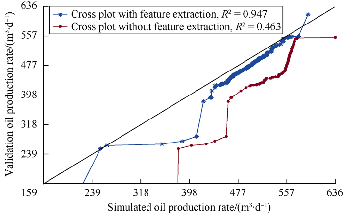
Fig. 12.
Cross-plot of simulated oil production rate and validation data.
Fig. 13.
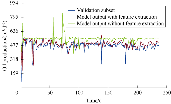
Fig. 13.
Comparison of actual oil production and simulated oil production.
Fig. 14.

Fig. 14.
Error distribution histogram of the oil production prediction model.
3.2. Architecture, training algorithm selection and validation of gas flow rate
A prediction model of gas flow rate was established by using the same procedure as the prediction model of oil flow rate. The same features previously extracted were used to improve the prediction performance of the model. The model was tested or validated by the data not used during the training process. Table 7 presents the information related to the optimum architecture of the model with feature extraction.
Table 7 Information related to the optimum architecture of ANN model for gas flow rate prediction.
| Items | Value/content |
|---|---|
| Number of inputs | 13 |
| Number of hidden Neurons | 15 |
| Output | Gas flow rate |
| Training algorithm | Bayesian regularization |
| R2 (Training) | 0.949 |
| R2 (Testing) | 0.971 |
| Number of epochs | 844 |
| Training time | 96 s |
A cross plot shown in Fig. 15 shows R2 values of the models with feature extraction and without feature extraction are 0.971 and 0.812 respectively. The predicted gas rates by the neural network model without feature extraction are higher than the actual production rates for most of the times, while the predicted gas production by the neural network model with feature extraction is the same with the actual gas produc- tion in most cases. This proves again that the physics based feature extraction adopted in this work has improved the prediction performance of the neural network model. It can be seen from Fig. 16 that the simulated results of the model with feature extraction are closer to the data in the validation subset. Besides, the error distribution histogram shown in Fig. 17 has a normal distribution trend, indicating that the mean error of the model is close to zero and the discrepancy is largely the result of measurement error.
Fig. 15.
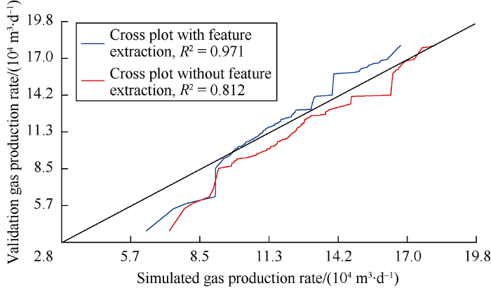
Fig. 15.
Cross-plot of simulated gas production and validation data.
Fig. 16.
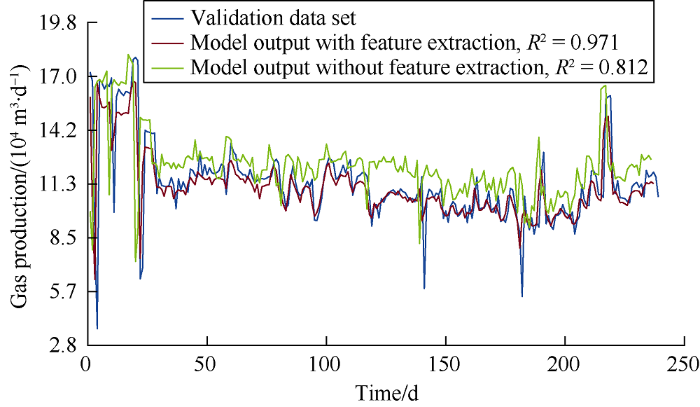
Fig. 16.
Comparison of actual gas production rate and simulated gas production rates.
Fig. 17.
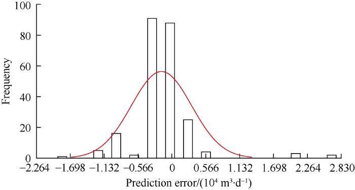
Fig. 17.
Error distribution histogram of the gas production model.
3.3. Architecture, training algorithm selection and validation of water flow rate
A similar approach used to design the oil production model was adopted to establish the water production prediction model. Table 8 presents the information related to the optimum architecture of the model with feature extraction.
Table 8 The information related to the optimum architecture of the ANN model for water production prediction.
| Item | Value/content |
|---|---|
| Number of inputs | 13 |
| Number of hidden neuron | 10 |
| Output | Water flow rate |
| Training algorithm | Bayesian regularization |
| R2 (Training) | 0.965 |
| R2 (Testing) | 0.971 |
| Number of epochs | 589 |
| Training time | 85 s |
The cross-plot in Fig. 18 shows that the R2 values of the models with and without feature extraction are 0.947 and 0.463 respectively. Fig. 19 shows that the results from the model with feature extraction are closer to the data in the validation subset than the results from the model without feature extraction. Besides, the error distribution histogram in Fig. 20 also shows a normal distribution trend, suggesting that the discrepancy is mainly due to measurement error.
Fig. 18.
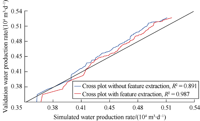
Fig. 18.
Cross-plot of predicted water production and validation data.
Fig. 19.
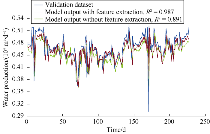
Fig. 19.
Comparison of actual water production and simulated water production.
Fig. 20.
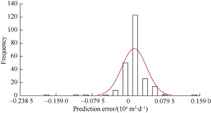
Fig. 20.
Error distribution histogram of the water production model.
4. Conclusions
Artificial neural network models were developed to predict oil, gas and water production rates of a water flooding reservoir. Unlike traditional models, neural network models need small amount of readily available information during the training of the selected architecture. Feature extraction and expansion based on the physics of reservoir flow and random combination of variables was used as a unique approach to improve prediction performance of the model. A neural network architecture trained by the Bayesian regularization is found to provide the smallest mean square error and the highest coefficient of determination during the training and validation of the selected neural network architecture. This algorithm typically takes longer time, but can result in good generalization of noisy datasets such as the oil, gas and water production rates used in this study. Moreover, the error distribution histogram was used to analyze the discrepancy between simulated output and validation data. The results show the errors of the models are most likely due to measurement.
Among all the features, the delay in time step term can improve the prediction performance of the models. This finding is of great significance, as many of prediction methods of the production during secondary recovery, including numerical reservoir modelling, do not take account of the past injection rate as a factor influencing current production rate.
Nomenclature
b—deviation;
d—delayed time steps;
f—NARX network architecture;
m, n—number of time steps;
t—serial number of time step;
u(t+1), u(t), ..., u(t-m)—external input data;
W—weight;
y(t), y(t-1), ..., y(t-n)—observation data;
y(t+1)—predicted value by the model;
σ—standard deviation.
Reference
Using least square support vector machines to approximate single phase flow
Artificial neural network and inverse solution method for assisted history matching of a reservoir model
Uncertainty assessment in production forecasting and optimization for a giant multi-layered sandstone reservoir using optimized artificial neural network technology
Application of artificial neural networks for calibration of a reservoir model
DOI:10.3233/IDT-180337 URL [Cited within: 1]
History matching of the PUNQ-S3 reservoir model using proxy modeling and multi-objective optimizations
An iterative response-surface methodology by use of high-degree-polynomial proxy models for integrated history matching and probabilistic forecasting applied to shale-gas reservoirs
Predicting waterflooding performance in low-permeability reservoirs with linear dynamical systems
Inferring interwell connectivity using production data
Technology focus: Petroleum data analytics
DOI:10.2118/1017-0087-JPT URL [Cited within: 1]
Data mining in cloud usage data with Matlab’s statistics and machine learning toolbox
Ensemble machine learning: An untapped modeling paradigm for petroleum reservoir characterization
DOI:10.1016/j.petrol.2017.01.024 URL [Cited within: 1]
Evaluation of machine learning methods for formation lithology identification: A comparison of tuning processes and model performances
DOI:10.1016/j.petrol.2017.10.028 URL [Cited within: 1]
Machine learning as a reliable technology for evaluating time/rate performance of unconventional wells
Data driven production forecasting using machine learning
Decline curve analysis for production forecasting based on machine learning
Data-driven optimization of injection/production in waterflood operations
Prediction of PVT properties in crude oil using machine learning techniques (MLT)
Petrophysical well log analysis through intelligent methods
An AI-based workflow for estimating shale barrier configurations from SAGD production histories
Prediction of void fraction for gas-liquid flow in horizontal, upward and downward inclined pipes using artificial neural network
DOI:10.1016/j.ijmultiphaseflow.2016.08.004 URL [Cited within: 1]
Integration of artificial intelligence and production data analysis for shale heterogeneity characterization in steam-assisted gravity-drainage reservoirs
DOI:10.1016/j.petrol.2017.12.046 URL [Cited within: 1]
MATLAB deep learning: With machine learning, neural networks and artificial intelligence
A new model selection strategy in time series forecasting with artificial neural networks: IHTS
DOI:10.1016/j.neucom.2015.10.036 URL [Cited within: 2]
Combining feature extraction and expansion to improve classification based similarity learning
DOI:10.1016/j.patrec.2016.11.005 URL [Cited within: 1]
Chaos time-series prediction based on an improved recursive levenberg-marquardt algorithm
DOI:10.1016/j.chaos.2017.04.032 URL [Cited within: 2]
Improvement of Levenberg- Marquardt algorithm during history fitting for reservoir simulation
DOI:10.1016/S1876-3804(16)30105-7 URL [Cited within: 1]
Reservoir zone prediction using logging data - multi well based on levenberg- marquardt method
Macau: Scalable Bayesian factorization with high-dimensional side information using MCMC
Uncertainty assessment in production forecast with an optimal artificial neural network
Assessment of data- driven, machine learning techniques for machinery prognostics of offshore assets
Performance forecasting for polymer flooding in heavy oil reservoirs
DOI:10.3390/polym10111225
URL
PMID:30961150
[Cited within: 1]

The flow of polymer solution and heavy oil in porous media is critical for polymer flooding in heavy oil reservoirs because it significantly determines the polymer enhanced oil recovery (EOR) and polymer flooding efficiency in heavy oil reservoirs. In this paper, physical experiments and numerical simulations were both applied to investigate the flow of partially hydrolyzed polyacrylamide (HPAM) solution and heavy oil, and their effects on polymer flooding in heavy oil reservoirs. First, physical experiments determined the rheology of the polymer solution and heavy oil and their flow in porous media. Then, a new mathematical model was proposed, and an in-house three-dimensional (3D) two-phase polymer flooding simulator was designed considering the non-Newtonian flow. The designed simulator was validated by comparing its results with those obtained from commercial software and typical polymer flooding experiments. The developed simulator was further applied to investigate the non-Newtonian flow in polymer flooding. The experimental results demonstrated that the flow behavior index of the polymer solution is 0.3655, showing a shear thinning; and heavy oil is a type of Bingham fluid that overcomes a threshold pressure gradient (TPG) to flow in porous media. Furthermore, the validation of the designed simulator was confirmed to possess high accuracy and reliability. According to its simulation results, the decreases of 1.66% and 2.49% in oil recovery are caused by the difference between 0.18 and 1 in the polymer solution flow behavior indexes of the pure polymer flooding (PPF) and typical polymer flooding (TPF), respectively. Moreover, for heavy oil, considering a TPG of 20 times greater than its original value, the oil recoveries of PPF and TPF are reduced by 0.01% and 5.77%, respectively. Furthermore, the combined effect of shear thinning and a threshold pressure gradient results in a greater decrease in oil recovery, with 1.74% and 8.35% for PPF and TPF, respectively. Thus, the non-Newtonian flow has a hugely adverse impact on the performance of polymer flooding in heavy oil reservoirs.
System identification based proxy model of a reservoir under water injection
