


Introduction
Despite continuous advancements in computational hardware technology, the gap between the available computational hardware and the required computational power for solving practical problems in engineering and science fields remains a concern. A real-time simulation is very high in computational cost. In computational engineering and science, proxy (or surrogate) models offer a computationally cheap alternative to high-fidelity models[1,2]. Although the practice of building proxy models is not new[1], in recent years more efforts have been made to employ machine learning algorithms to approximate the results of Computational Fluid Dynamics models[2]. With the development of modern hardware like GPUs (Graphics Processing Units), sophisticated deep learning techniques are making their way into proxy modeling efforts. That proxy models have been utilized in other fields such as material science[3], computational solid mechanics[4], weather modeling[5], life science[6], computational physics[7], and computational chemistry[8]. For the most of these applications, proxy models are developed based on a supervised learning approach. In this approach, machine learning models are trained based on a database generated from a few scenarios ran by the basic simulation model[2, 9-10].
In subsurface modeling and the earth science domain, one approach is to utilize proxy modeling as a facilitator to numerical physics-based approaches such as numerical reservoir simulation models. Reservoir simulation models constitute the standard modeling tools utilized by the oil and gas industry to understand the fluid flow behavior in porous media under certain operational conditions. These models are widely used in the petroleum reservoir management workflows for purposes such as forecasting well production, optimizing injection scenarios, proposing infill wells, understanding the communications between wells/reservoirs, etc. A calibration (history matching) process is usually conducted by the engineering and subsurface team to make the reservoir model trustworthy[11]. A calibrated model then is used to study different operational scenarios, to analyze the sensitivity of input and output data, and to assess the uncertainty involved in the operational decisions. Such tasks require a large number of realizations from the base reservoir simulation models. These models are usually computationally expensive and time-consuming to run. Therefore, a realistic subsurface modeling study is not able to take full advantage of reservoir simulation models’ capabilities. In this paper we argue that the development of smart proxies for reservoir simulation models would help the reservoir management team to utilize the capabilities of reservoir simulation models at a very low computational cost.
Artificial neural networks (ANNs) have been widely employed to develop proxy models for the purpose of petroleum reservoir management. Despite the black box characteristic of ANNs, they are capable of learning the non-linear patterns behind complex databases, which makes them suitable for many problems in the subsurface domain. Examples of ANNs’ applications in reservoir management workflow are production forecast[12], well placement, anomaly detection, and steam injection optimization, etc. In this paper we look into two case studies of ANN applications for subsurface modeling. The first case study involves building a proxy model using ANNs for the purpose of estimating well pressure and production, and focuses on history matching. The second case study demonstrates the ability of ANNs for fast-track prediction of reservoir behavior such as phase saturation and pressure distribution in a specific formation. The databases for both case studies are available in references [13-14]. When compared to results given by using blind databases, the results of the two proxy models underscore the strength of ANNs when utilized for fast-track modeling of the subsurface.
1. Materials and methods
The general machine learning workflow for developing a data-driven proxy model is described in Fig. 1. With the help of subject expert matter, the data scientist/engineer needs to understand the problem and the available data thoroughly. In conventional machine learning and pattern recognition approaches, the pre-processing step requires the extraction of reservoir features from the available raw data. This step helps cleanse, process, and derive additional values from the original data, and is necessary in order to eliminate redundant data in the database prior to the model development step. The feature extraction step highly benefits from the knowledge of the domain expert. Subsequent databases will be used to develop the machine learning models. The choice of machine learning algorithms mostly relies on the quality and volume of available data and the goal of project. For the two case studies described below, we used artificial neural networks (feed- forward ANNs) mainly for their abilities to understand the complex and non-linear data types and their tolerance to noisy data. We also preferred ANNs given their generalization capability. A review of ANN capabilities and applications in petroleum engineering can be found in reference [15].
Fig. 1.
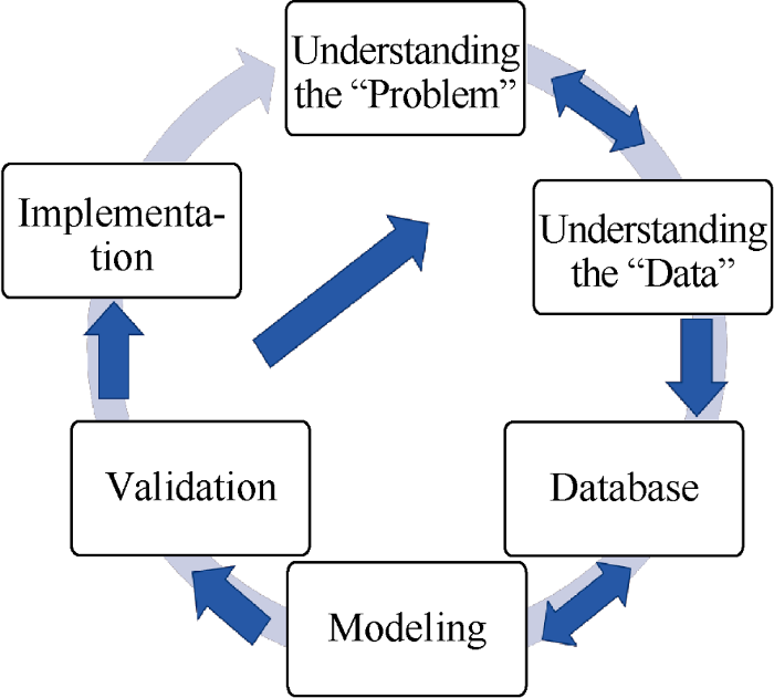
Fig. 1.
A data-driven modeling workflow.
The process to develop a proxy model for reservoir geologic model generally includes designing basic reservoir numerical simulation, building time-space database, feature selection, building machine learning model, blind test and analysis by using the proxy model. The proxy model can serve as approximation of full-field 3D numerical reservoir simulation model. Once the goals of the two studies were set, we designed and ran a few scenarios of the base reservoir simulation model. The design of the experiment (DOE) sampling techniques (such as Latin Hypercube) has been used in this step to cover the uncertainty in the solution space. The initial number of simulation runs is typically subjective. If this number is too large, it will not justify the application of the proxy model. At the same time, a very small number of simulation runs will present limited information to build a robust proxy model. Based on the authors’ experience with such models, 10 to 16 simulation runs constitutes a good start for subsurface modeling projects, if the base model includes enough heterogeneity. As described in Fig. 1, if a model fails the validation step, a new set of simulation runs should be added to the database. For instance in the first case study, we chose ten simulation runs for training the proxy model and an extra simulation run was utilized for validating the trained proxy model (blind verification). This number of runs led to an accurate proxy model. For the second case study initially ten and three simulation runs were used for training and validation (blind verification), respectively. However, a specific proxy model for predicting water saturation did not result in satisfactory outcomes (less than 5% absolute error), therefore we did add six more simulation runs for this case.
Once we set the initial number of informative simulation runs, the raw data was extracted to build the spatiotemporal database. In general, the goal of the study influences the feature selection and the parameterization of data. In the next section, we will discuss two case studies whose goals are distinct and therefore show the flexibility of proxy modeling for subsurface modeling applications. If the first study aims to estimate well production and pressure, the second case aims to predict areal pressure and phase saturations. Because of the nature of the outputs, we call the first case study a well-based proxy modeling and the second case, a grid-base proxy modeling. Subsequently, each case study requires its own feature selection approach and parameter representation.
During the ML model and proxy model development, the data engineer must avoid overfitting. An overfit model shows a strong performance on the training database; however, it is not generalized enough to perform well on an unforeseen data set. Two approaches can be used to avoid overfitting. First, during the training step, the data engineer could monitor the error trend of training and testing sets. Fig. 2 depicts how to choose a fit model during the training step. Second, the data engineer can do a blind dataset verification. Once a model is trained, it is important to validate it against unforeseen data. The “blind” validation step ensures that the models are not overfit and can perform well on a set of unforeseen data.
Fig. 2.
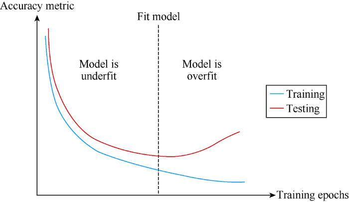
Fig. 2.
Comparison of training and testing errors in order to avoid an overfit model.
2. Results
2.1. Case study one: Smart proxy for assisted history matching
This first case study investigates the application of a proxy model for calibrating a reservoir simulation model based on historical data. A standard reservoir simulation model known as PUNQ-S3[16] was used for this purpose. This reservoir simulation model was adapted from a real reservoir and is known and utilized in petroleum engineering literature for testing the capabilities of history matching and uncertainty quantification methods. The proxy model was developed using a small number of PUNQ-S3 geological realizations. We considered the following uncertain properties: distributions of porosity, horizontal permeability, and vertical permeability. Several ANNs comprised the predictive engine of our proxy model. The trained proxy model was tested against unforeseen realizations of the simulation model (in a process called “blind verification”). Next, the validated proxy model was coupled with an evolutionary optimization algorithm known as Differential Evolution (DE)[11, 15] to conduct automated history matching.
The PUNQ-S3 reservoir model includes five geological layers, each containing 19 by 28 grid blocks (180 m by 180 m). The reservoir is surrounded by a fault to the east and south and is supported by an underlaying aquifer. Its pressure is below bubble point; a gas cap is present in the reservoir’s top layer. Six production wells were drilled in this reservoir, and the initial values of water-oil-contact (WOC) and gas-oil- contact (GOC) depths were reported. Fig. 3 shows the top structure of this reservoir, the fault lines, the WOC contour line, the GOC contour line, and the well locations. In order to avoid excess gas production, the top two layers were left without perforation. The other layers were completed in the following orders: wells PRO-1, PRO-4, and PRO-12 were completed in layers 4 and 5; wells PRO-5 and PRO-11 were perforated in layers 3 and 4; and well PRO-15 was only perforated in layer 4. Fig. 4 shows the “true” distributions of permeability (vertical and horizontal) and porosity. The base reservoir simulation model was borrowed from reference [17] and it was rebuilt in CMG format[18]. Following is the list of the available data:
$\bullet$ Porosity and permeability values at well locations
$\bullet$ Geological descriptions for each layer
$\bullet$ Production history for the first 8 years (for history matching purpose)
$\bullet$ Cumulative production after 16.5 years
$\bullet$ PVT, relative permeability, and Carter- Tracy aquifer dataset, all taken from the original field data
$\bullet$ No capillary function
$\bullet$ GOC and WOC
Fig. 3.

Fig. 3.
The top structure of PUNQ-S3 model[16].
Fig. 4.
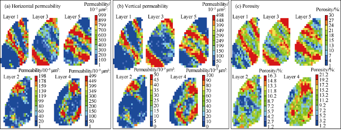
Fig. 4.
“True” distributions of porosity and permeability are provided for PUNQ-S3 reservoir model.
The base reservoir simulation model PUNQ-S3[18] was used as a benchmark for generating a few informative realizations of the reservoir model. Based on the property values provided at the well sites and the geological descriptions, eleven different realizations of the reservoir were created by using the experiment design method called the Latin Hypercube. A detailed discussion on generating these realizations is available in reference [15]. Ten realizations of the reservoir were used for training the ANNs, while the eleventh realization was used for blind validation of the trained model.
Different types of data were extracted from the simulation runs to form a spatiotemporal database. This database included the inputs and outputs for training the ANNs. The input data includes coordinates of the well locations, top depth, porosity, horizontal and vertical permeabilities, thickness, oil production and the output of the previous time step. The outputs include bottom-hole pressure, gas production and water production. In order to reduce the dimension of the problem and simplify the data for training the ANNs, we adopted the segmentation and tiering system depicted in Fig. 5a shows the well-based reservoir segmentation, modified from the Voronoi diagrams[19,20]. In this system, each well is assigned a drainage area generated using the modified Voronoi theory. In Fig. 5b, each drainage area is divided into four tiers. Considering the significant impact of the surrounding area around the well block on well production, the first tier only includes the well block. The second and third tiers consist of the first and second rows of grid blocks around the well block, respectively. Finally, the fourth grid sums up the remaining grid blocks in the drainage area. The average values of reservoir properties such as top depth, thickness, porosity, and permeability were calculated at each tier and allocated to the corresponding well and tiers in the database.
Fig. 5.
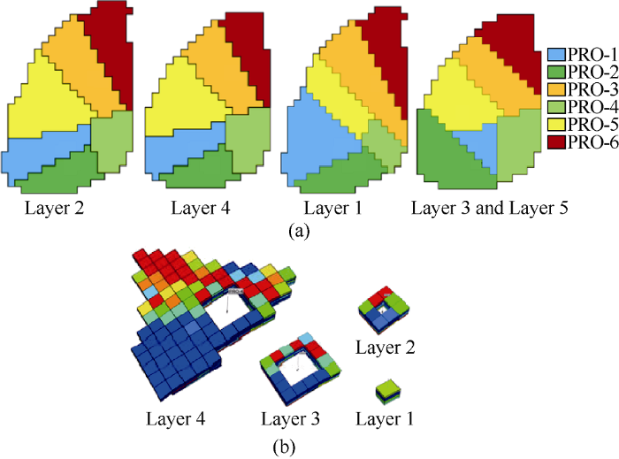
Fig. 5.
Designed segmentation of the PUNQ-S3 reservoir model. (a) well-based drainage area segmentation. (b) the tier system for each drainage area.
Corresponding to the number of outputs (well bottom-hole pressure, gas production rate, and water production rate), the final version of our proxy model comprised three ANNs. The inputs and corresponding outputs for each ANN in this study included the coordinates of the grids the wells are, top depth, porosity, horizontal and vertical permeability, thickness, and oil production rate of each layer (5 geological layers and 4 grid layers), output of the previous time step and time. The outputs included bottom-hole pressure, gas and water production rates. Each well (and its corresponding segmentation) has 60 uncertain parameters (5 geological layer × 4 tiers × 3 uncertain properties). Therefore, the total number of uncertain parameters we used to fine-tune the matching model was 360, which included 5 geological layers × 4 tiers × 6 wells × 3 properties. In addition to these uncertain parameters, other information such as metadata, geological characteristics, well locations, and operational constraints were included in the database.
In training the ANNS, we divided the database into three sets: 80% of it represented the segment used for training, 10% of the database was used for calibration, and 10% for validation. Each ANN had one hidden layer. The number of hidden layers and hidden neurons, and the learning rate of each ANN constitute the hyperparameters that could be adjusted to optimize the learning process. However, in this study we focused on data representation alone and used the default values.
Once the ANNs were trained and validated (using the extra scenario), they gave shape to the proxy model used for conducting the assisted history matching. A well-built proxy model is capable of taking the reservoir characteristics and production constraints (oil production rate at each time step) and estimate the values of outputs (well bottom-hole pressure, gas rate, water rate). Having obtained the output values at each time step, we were able to compare them with their historical values and to estimate their objective function (loss function).
For this study, we utilized a version of the root mean square error (RMSE) to evaluate the error between the estimated and actual values. Equation 1 estimates the relative differences at the well level. The weighting factor gives the user options to adjust the objective function based on the importance of data. For instance, if a particular well (or a time period) is more significant in the production portfolio, the user might consider adjusting the weight coefficients to include the importance of this well. In order to have a metric in a field-level, we used Equation 2 that defines a global objective function including all the wells. This equation describes the global objective function using the well level objective function, which we defined in Equation 1. In this study, we consider all the wells and measured data points being equally important and the weighting factors being equal to one.
The results of our validation set and history matching for a limited number of wells are shown in Figs. 6-8. Fig. 6 shows the results of the validation dataset calculated by the proxy model and the reservoir simulation model, including well bottom-hole pressure, gas production rate, and water production rate. The results of the validation .set underscore the strength of trained ANNs for predicting a set of data that was not used during the training step. Fig. 7 shows the results of the history matching process considering well bottom-hole pressure and gas production for wells PRO-1 and PRO-4. Because of the non-uniqueness characteristics of the history matching process, we considered the results of the ten best matches. The ten best matches represent the outcome of the coupling the proxy model and Differential Evolution optimization algorithm. In general, the history match results for well bottom-hole pressure and gas rate were very good.
Fig. 6.
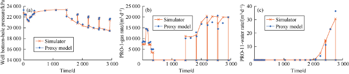
Fig. 6.
Comparison of well bottom-hole pressure, gas production rate, and water production rate results from the proxy model and reservoir simulation model for the validation dataset (blind verification run).
Fig. 7.
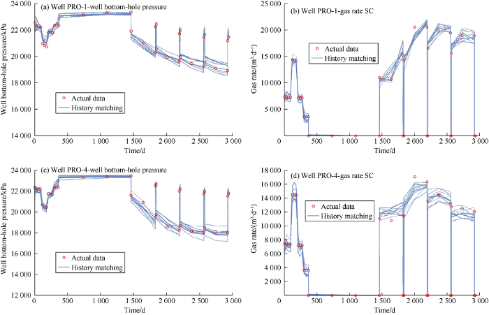
Fig. 7.
History matching results of well bottom-hole pressure and gas production rate for wells PRO-4 and PRO-1.
Fig. 8.
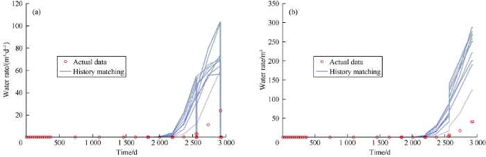
Fig. 8.
History matching results of water production rate and cumulative water production of well PRO-11.
2.2. Case study two: Smart proxy for fast-track modeling of CO2 enhanced oil recovery and storage
The second case in this paper investigated the application of an ANN-based proxy model for fast-track modeling of CO2 enhanced oil recovery. If in the previous case study, the proxy model generated results of the numerical reservoir simulation model at the well level, in this case, we aimed to approximate the outputs of the reservoir simulation model at the grid block level. The study aimed to examine the consequences of uncertainty in the reservoir characteristic (permeability at the grid block) and the sensitivity of operational constraints (injection well bottom-hole pressure) on the behavior of pressure and phase saturations.
The detailed reservoir simulation study is available in reference [21]. The secondary objective of the reservoir simulation study was to investigate the scenario of 50 years of CO2 injection in an oil field and then monitor the movement of CO2 plume over a period of 1000 years. The original geo-cellular model in this work included over nine million grid blocks. In order to simulate the CO2 trapping mechanisms, we had to upscale the original model to 13 600 grid blocks. Even the upscaled version of the simulation model required a high computational cost and took hours to run a single scenario. The reservoir simulation in this study was conducted using a Computer Modeling Group (CMG) simulator called GEM-GHGTM[22].
The reservoir model belonged to SACROC Unit in the Kelly-Snyder field in West Texas. The SACROC Unit, within the Horseshoe Atoll, is the oldest continuously operated CO2 enhanced oil recovery operation in the United States, having undergone CO2 injection since 1972. Until 2005, about 93 million tons (93 673 236 443 kg) of CO2 had been injected and about 38 million tons (38 040 501 080 kg) had been produced. As a result, a simple mass balance suggests that the site has accumulated about 55 million tons (55 632 735 360 kg) of CO2[23,24].
The reservoir simulation model in this case study was built based on the work done by Han[25]. The original model simulated an enhanced oil recovery (EOR) process for a period of 200 years (1972-2172). We used the reservoir dynamic properties such as pressure and saturation distributions after 200 years of EOR to build our base reservoir simulation model. Our model aimed to simulate a 1000 years period (2172-3172), the first 50 years of which would include the CO2 injection.
Our reservoir model included 25 simulation layers of 16× 34 grid blocks. We considered the fact that 45 injection wells are already planned to inject CO2 at a constant rate (331 801.9 m3/day) for 50 years starting in 2172. Each well is perforated in a single layer, although the perforated layers might be different for different wells. The perforations happen in layers 19 (one well), 20 (40 wells), 21 (one well) and 22 (three wells). We assumed that there is no-flow boundary condition at the outer boundaries. Fig. 9 shows a three-dimensional view of the structure in this simulation model.
Fig. 9.
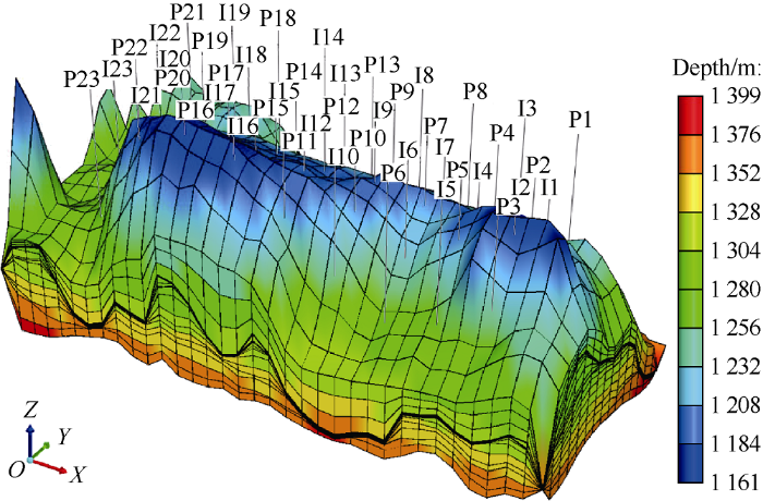
Fig. 9.
Top structure of SACROC Unit reservoir model.
We were interested in understanding the impact of the uncertainty of permeability distributions at nine layers (layers 1, 2, 19, 20, 21, 22, 23, 24, and 25) as well as the sensitivity of flowing bottom-hole pressure at 45 injection wells. We intended the reservoir model to track the distribution of pressure and phase saturations at the target layer (layer 18) during and after injection of CO2. Layer 18 was chosen to be monitored because of its location atop of the perforated layers. The total number of grid blocks in this layer is 544, of which only 422 grid blocks are active. The white grid blocks represent “null” or inactive blocks because they have a very low thickness. The initial condition we considered is the condition of the reservoir after 200 years of EOR process (from 1972 to 2172), which comes from the original model.
Fig. 10.
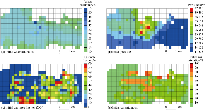
Fig. 10.
The initial dynamic reservoir properties (pressure, water saturation, gas saturation, and gas mole fraction [CO2]) at the target layer (layer 18).
In order to build the spatiotemporal database for training and validating the ANNs, we generated a few scenarios of the base reservoir simulation model. For each scenario, we modified the permeability values at nine layers (layers 1, 2, 19, 20, 21, 22, 23, 24, and 25) and the flowing bottom-hole pressure at 45 injection wells. We used the range of permeability in the base model for creating permeability distributions. Also, we used 60% to 100% of the litho-static pressure as the benchmark for generating the injection bottom-hole scenarios. An experimental design method (Latin Hypercube) was utilized over the properties range to construct combinations of the input parameter values, such that the maximum information that can be obtained from the minimum number of simulation runs. In the experimental design method, the range and average of permeability distribution was constrained to the base model. The distribution of permeability changed over different realizations. We assume that permeability values at the well locations are available (in reality coming from the core data); therefore, using a geo-statistical method (Inverse Distance Estimation provided in CMG-Builder), a distribution of permeability can be generated. Fig. 11 shows the process of generating new realizations (altering permeability distribution and BHP at injection wells).
Fig. 11.
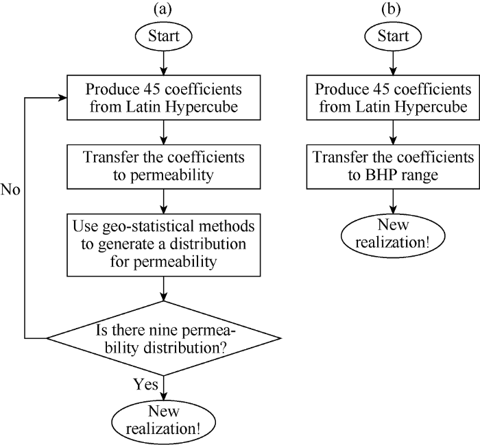
Fig. 11.
Flow charts for generating a new realization by changing the permeability distribution (Part a.) and altering flowing bottom-hole pressure at injection wells (Part b.).
The input list includes the static properties such as porosity, permeability, thickness, and top depth of grid block, as well as the dynamic properties (properties that are varying vs. time) such as operational constraint (injection bottom-hole pressure) and initial pressure and phase saturations. The outputs observed are the pressure and phase saturations at the grid block. We developed an ANN for each output property and combined the results of the ANNs to form the proxy model. We used 10 reservoir simulation runs to train the pressure ANN and 16 reservoir simulation runs for training the phase saturation ANNs. Three extra runs were used for the blind verification of the already trained ANNs. Fig. 12 displays the distributions of permeability for Layer 1, 2, 19, and 20 for 13 scenarios (10 for training, 3 for the blind verification). Fig. 13 also shows flowing bottom-hole pressure at the injection wells for 13 scenarios.
Fig. 12.

Fig. 12.
Distributions of permeability for layers 1, 2, 19, and 20 for 13 realizations. Ten realizations are used for training the proxy model and three realizations are used for validating the proxy model.
Fig. 13.
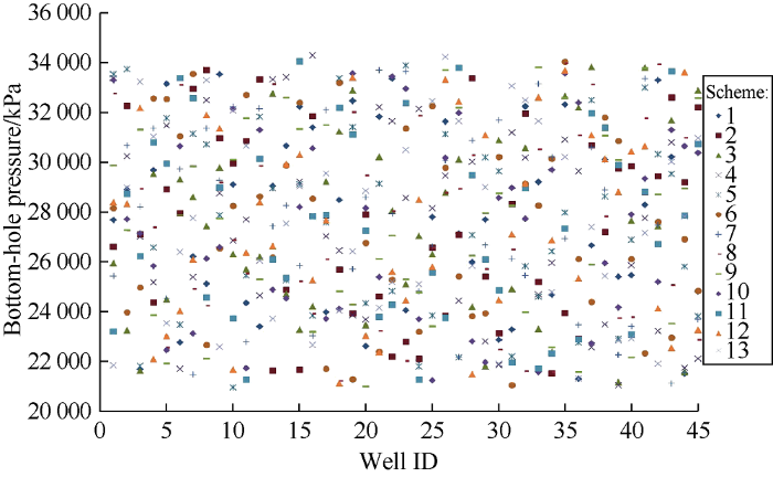
Fig. 13.
Flowing bottom-hole pressures in 45 injection wells from the ten training and three blind realizations.
The training and validation of the ANNs were accomplished using a software application called IDEATM[26]. IDEATM is typically used in the development of data-driven models for oilfield applications. One hidden layer was used for both case studies in this paper. The number of hidden neurons followed a rule of thumb of 2n-1, in which n represents the number of inputs. We used feed forward neural networks and backpropagation algorithm for training. Sigmoid activation function was the default activation algorithm in IDEATM. Also IDEATM dynamically chose the learning rates. As highlighted above, the spatiotemporal database was built based on the information from 10 (10 for pressure distribution and 16 for phase saturations) simulation runs. We divided the database into three segments: training (80%), calibration (10%), and verification (10%). After training three ANNs, we were able to verify their robustness using blind realizations. These runs were not used at any other step including training, calibration, or verification. In addition, we chose back-propagation as the algorithm for training the ANNs.
The pressure distributions in the target layer (layer 18) during and after the CO2 injection predicted by the proxy model are shown in Figs. 14 and 15. Fig. 14a-b shows the comparison of the pressure distribution predicted by the proxy model and the base model after 9 years of CO2 injection. Fig. 14c shows the relative error distribution between the results from the base model and the proxy model. Fig. 15 shows the pressure distribution 100 years after the injection ends predicted by a blind validation realization. A complete set of our simulation results including the training and verification realizations is available in reference [21]. As expected, the training results had a better performance than the blind validation sets. Our proxy model predicts the pressure distribution very well for a validation set.
Fig. 14.

Fig. 14.
Comparison between the results of simulation model and proxy for pressure distribution of a blind (validation) realization at layer 18, nine years after injection starts.
Fig. 15.

Fig. 15.
Comparison between the results of simulation model and proxy for pressure distribution of a blind (validation) realization at layer 18, 100 years after injection starts.
Figs. 16 and 17 present the comparison between the results of the simulation model and the proxy model for water saturation distributions at layer 18. Fig. 16 shows the results during the nine-year injection period, and Fig. 17 shows the results of a post injection time period (100 years after injection ends). Figs. 16c and 17c show the absolute error distributions between the simulation model and proxy model estimations. While the majority of absolute error values are less than 0.03 (3%), the maximum value of absolute error is less than 0.06 (6%).
Fig. 16.
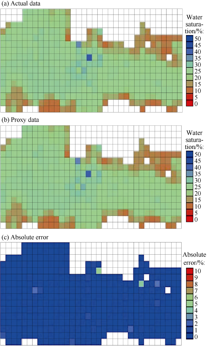
Fig. 16.
Comparison between the results of simulation model and proxy for water saturation distribution of a blind realization at layer 18, nine years after injection starts.
Fig. 17.

Fig. 17.
Comparison between the results of simulation model and proxy for water saturation distribution of a blind (validation) realization at layer 18, 100 years after injection ends.
Figs. 18 and 19 show the CO2 mole fraction distributions in the layer 18 nine years after the beginning of the injection and 100 years after the end of the injection predicted by the base model and proxy model. Figs. 18c and 19c show the absolution error distributions. Similar to the water saturation results, the majority of error values are less than 0.03 (3%). However, we observe a higher maximum value of absolute error (around 0.1 or 10%).
Fig. 18.
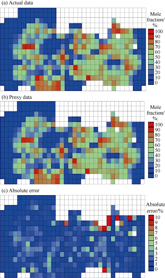
Fig. 18.
Comparison between the results of simulation model and proxy for gas (CO2) mole fraction distribution of a blind (validation) realization at layer 18, nine years after injection starts.
Fig. 19.

Fig. 19.
Comparison between the results of simulation model and proxy for gas (CO2) mole fraction distribution of a blind (validation) realization at layer 18, 100 years after injection ends.
3. Discussion
The computational cost associated with multi-scale and multi-phase reservoir simulation model renders the imple-mentation of reservoir simulation models in closed-loop reservoir management[27]. However, the machine learning based proxy models offer an alternative strategy. A successfully developed and validated proxy model is able to reproduce the results of the reservoir simulation model in fractions of the time and with very low computational costs for running a single realization of the original reservoir simulation model. In this paper we have shown the steps required to build successful proxy models for two case studies. Both case studies provide details and quantified results of subsurface behavior. However, the goals of these studies are different. The first cases study (PUNQ-S3 reservoir) aims to estimate the outputs at the well locations. The second case study (SACROC Unit reservoir) intends to predict the behavior of reservoir pressure and phase saturations during and after injection periods. In particular, we are interested in learning these behaviors at different time periods and spaces across the reservoir.
These two case studies provided opportunities to test the robustness of the proxy modeling application for reservoir studies. There are a few points to discuss here. The first point is the computational cost advantage in developing and using proxy models versus the original simulation runs. The PUNQ-S3 reservoir model was a black oil model, and the run-time for a single simulation was less than five minutes on a cluster of twelve 3.2 GHz processors. In order to build the proxy model, we used 11 (10 for training and 1 for validation) realizations of the base reservoir simulation model. The validated proxy model had the run-time of less than a second for each run. The automated history matching workflow was constructed by setting up the misfit functions (Equation 1 and Equation 2) and utilizing an optimization algorithm (DE) for tuning the uncertain parameters. Our stoppage criterion was 1000 calls of proxy model and misfit calculations. The call of proxy model, misfit calculations, and the implementation of the DE algorithm took about a second for each run on a cluster of twelve 3.2 GHz processors. The history matching outputs discussed in the results section were achieved in almost 1000 seconds. In addition, the run-time for running the eleven realizations of the base model was 3300 seconds (11 realizations, on average 5 minutes for each run). Therefore, the total cost for the development, validation, and deployment of the proxy model for history matching in the PUNQ-S3 reservoir model was 4300 seconds. If we were to use the PUNQ-S3 reservoir simulation model in the same history matching workflow and with the same stoppage criterion (1000 calls), we would have required 300 000 seconds of computational time (1000 realizations and 5 minutes average run-time for each realization). By using the proxy model, we saved 98.9% of computational time. The SACROC Unit reservoir model had a much higher run-time. Using the cluster of twelve 3.2 GHz processors on average took 10-24 hours (depending on computational convergence for some space and time steps) for each realization of the reservoir simulation model. On the contrary, the results of our study detailed in the section above were produced using the proxy model in a less than a few seconds.
We used ANNs for developing our proxy models. However, ANNs are not the only machine algorithms available for proxy modeling applications. Reasons to choose ANNs for supervised learning (when our data is labeled, and labels are provided during the training step.) include their high predic-tive accuracy, their capability to learn the main signal, and their ability to learn the non-linear behavior of data. Nevertheless, ANNs have some limitations. For instance, the black-box nature of the ANNs limits the interpretability of results and algorithm. Also, the training pace of ANNs relative to the implementation speed is slow. Another limitation is the high number of hyperparameters (such as the number of hidden layers, the number of hidden neurons, and the learning rate) that might impact the accuracy of the trained model. In terms of prediction accuracy, relatively newer machine learning techniques such as Support Vector Machines (SVMs) and boosting algorithms (like Adaptive Boosting) have better performance than ANN[28]. There are other supervised learning algorithms that could perform better than ANNs for the specific limitations mentioned earlier. For instance, when it comes to result interpretability, algorithms such as Decision Trees, Random Forests, and Regression models do well. The training pace for Decision Trees and Regression models is fast, although they do not suit non-linear problems. For the hyper-parameter selection, one might perform a search only changing these parameters and compare the results to choose the best set of hyper-parameters. The Genetic Algorithm[29] and the Bayesian Optimization[30] are the most commonly used techniques to auto-tune the hyper-parameters. It should be noted that we chose not to tune the hyper-parameters of our ANNs (the number of hidden layers, number of hidden neurons, and learning rate) in the two case studies. If one chooses to tune the hyper-parameters, the training time of ANNs could increase significantly.
Another point to consider is the number of simulation runs required to build the proxy model. The data in the spatiotemporal database originates from informative simulation runs. There are no rules to identify the exact number of runs required to build a perfect proxy model. Performing a sensitivity analysis on the accuracy of the proxy model versus the number of simulation runs could be useful. The complexity of the reservoir model and heterogeneity may affect the number of required runs. Based on the authors’ experience, a homogeneous reservoir requires a higher number of runs than a more complex and heterogeneous reservoir. We can relate this to the higher level of information provided in a heterogeneous reservoir when compared to a homogenous reservoir. Also, data parameterization is key in reducing the dimensionality of the problem. In the first case study (PUNQ-S3 reservoir), we used the Voronoi graph theory[19,20] and a tiering system to parameterize the reservoir and reduce the number of parameters. More creativity in the representation and summarization of the data would be beneficial.
4. Conclusions
Although we encourage their use as a solid guideline, the steps to build proxy models described in this paper will not serve as a one-size-fits-all in developing any proxy models. On the contrary, due to the nature of subsurface problems, data engineers and scientists should pay extra attention to the preprocessing steps, feature selection, and model selection. However, the results of this study prove the ability of machine learning-based proxy models, as fast and accurate tools improving the performance of reservoir simulation models. The results of this study also benefit the other time-consuming operations in the reservoir management workflow such as sensitivity analysis, production optimization, and uncertainty assessment.
Acknowledgements
The authors would like to thank Intelligent Solutions Inc. for providing the software package used in developing the proxy models. The authors would also like to thank Computer Modeling Group for providing access to the numerical reser-voir simulation software.
Nomenclature
Fglobal—global objective function;
Fi—objective function of well i;
N(i)—the number of parameters need to be matched (for example, oil, gas and water production rates);
Nt(i,j)—total time step;
Nw—total number of wells;
Ys,i,j,t—production predicted by the proxy model, m3/d;
Ym,i,j,t—actual production, m3/d;
wt—weight factor, dimensionless;
ΔYm,i,j—the difference between the maximum and minimum measured data of well i, m3/d.
Subscript:
i—Well No.;
j—Property No.;
t—time step.
Reference
Application of machine learning algorithms to flow modeling and optimization
Data driven smart proxy for CFD application of big data analytics & machine learning in computational fluid dynamics, part three: Model building at the layer level
(
Machine learning in materials informatics: Recent applications and prospects
DOI:10.1038/s41524-017-0056-5 URL [Cited within: 1]
A finite element-based machine learning approach for modeling the mechanical behavior of the breast tissues under compression in real-time
DOI:10.1016/j.compbiomed.2017.09.019
URL
PMID:28982035
[Cited within: 1]

This work presents a data-driven method to simulate, in real-time, the biomechanical behavior of the breast tissues in some image-guided interventions such as biopsies or radiotherapy dose delivery as well as to speed up multimodal registration algorithms. Ten real breasts were used for this work. Their deformation due to the displacement of two compression plates was simulated off-line using the finite element (FE) method. Three machine learning models were trained with the data from those simulations. Then, they were used to predict in real-time the deformation of the breast tissues during the compression. The models were a decision tree and two tree-based ensemble methods (extremely randomized trees and random forest). Two different experimental setups were designed to validate and study the performance of these models under different conditions. The mean 3D Euclidean distance between nodes predicted by the models and those extracted from the FE simulations was calculated to assess the performance of the models in the validation set. The experiments proved that extremely randomized trees performed better than the other two models. The mean error committed by the three models in the prediction of the nodal displacements was under 2 mm, a threshold usually set for clinical applications. The time needed for breast compression prediction is sufficiently short to allow its use in real-time (<0.2 s).
Weather forecasting model using artificial neural network
DOI:10.1016/j.protcy.2012.05.047 URL [Cited within: 1]
Analysis of deep learning method for protein contact prediction in CASP12
Accelerating science with generative adversarial networks: An application to 3D particle showers in multilayer calorimeters
DOI:10.1103/PhysRevLett.120.042003
URL
PMID:29437460
[Cited within: 1]
Physicists at the Large Hadron Collider (LHC) rely on detailed simulations of particle collisions to build expectations of what experimental data may look like under different theoretical modeling assumptions. Petabytes of simulated data are needed to develop analysis techniques, though they are expensive to generate using existing algorithms and computing resources. The modeling of detectors and the precise description of particle cascades as they interact with the material in the calorimeter are the most computationally demanding steps in the simulation pipeline. We therefore introduce a deep neural network-based generative model to enable high-fidelity, fast, electromagnetic calorimeter simulation. There are still challenges for achieving precision across the entire phase space, but our current solution can reproduce a variety of particle shower properties while achieving speedup factors of up to 100 000×. This opens the door to a new era of fast simulation that could save significant computing time and disk space, while extending the reach of physics searches and precision measurements at the LHC and beyond.
Deep learning for computational chemistry
DOI:10.1002/jcc.23255
URL
PMID:23483582
[Cited within: 1]
A valence-universal multireference coupled cluster (VUMRCC) theory, realized via the eigenvalue independent partitioning (EIP) route, has been implemented with full inclusion of triples excitations for computing and analyzing the entire main and several satellite peaks in the ionization potential spectra of several molecules. The EIP-VUMRCC method, unlike the traditional VUMRCC theory, allows divergence-free homing-in to satellite roots which would otherwise have been plagued by intruders, and is thus numerically more robust to obtain more efficient and dependable computational schemes allowing more extensive use of the approach. The computed ionization potentials (IPs) as a result of truncation of the (N-1) electron basis manifold involving virtual functions such as 2h-p and 3h-2p by different energy thresholds varying from 5 to 15 a.u. with 1 a.u. intervals as well as thresholds such as 20, 25, and 30 a.u. have been carefully looked into. Cutoff at around 25 a.u. turns out to be an optimal threshold. Molecules such as C2H4 and C2H2 (X = D,T), and N2 and CO (X = D,T,Q) with Dunning's cc-pVXZ bases have been investigated to determine all main and 2h-p shake-up and 3h-2p double shake-up satellite IPs. We believe that the present work will pave the way to a wider application of the method by providing main and satellite IPs for some problematic N-electron closed shell systems.
Data- driven fluid simulations using regression forests
Data-driven projection method in fluid simulation
Assisted history matching using pattern recognition technology
Application of machine learning algorithms for optimizing future production in Marcellus shale: Case study of southwestern Pennsylvania
Database for PUNQ-S3 case study
(
Database for PUNQ-S3 case study
(
Artificial intelligence assisted history matching: Proof of concept. Morgantown,
Methods for quantifying the uncertainty of production forecasts
Standard models: PUNQ-S3 model
.[
PUNQ-S3 reservoir model (CMG format) for history matching study
(
The graph Voronoi diagram with applications
DOI:10.1002/(ISSN)1097-0037 URL [Cited within: 2]
Top down intelligent reservoir modeling
Modeling pressure and saturation distribution in a CO2 storage project using a surrogate reservoir model (SRM)
DOI:10.1002/ghg.1414 URL [Cited within: 2]
Advanced compositional reservoir simulator
.[
Kelly-Snyder fields/SACROC unit
Smart proxy modeling of SACROC CO2-EOR
DOI:10.1007/s11136-017-1779-y
URL
PMID:29357027
[Cited within: 1]
Acute respiratory infections (ARIs), and associated symptoms such as cough, are frequently experienced among children and impose a burden on families (e.g., use of medical resources and time off work/school). However, there are little data on changes in, and predictors of, quality of life (QoL) over the duration of an ARI with cough (ARIwC) episode. We therefore aimed to determine cough-specific QoL and identify its influencing factors among children with ARIwC, at the time of presentation to a pediatric emergency department (ED), and over the following 4 weeks.
Evaluation of CO2 trapping mechanisms at the SACROC northern platform: Site of 35 years of CO2 injection
IDEATM
[
Production management decision analysis using AI-based proxy modeling of reservoir simulations: A look-back case study
An empirical comparison of supervised learning algorithms
A genetic programming approach to designing convolutional neural network architectures
Practical Bayesian optimization of machine learning algorithms
