


Introduction
Production profile logging is an important way of monitoring the dynamics in oil and gas field development, and one of the important supporting technologies for horizontal well development[1]. It is of great significance for adjusting the development plan of oil field, keeping the oil well in the best production state, and enhancing oil recovery. In production logging, the fluid flow parameters of each well are measured dynamically, then the flow rates of different phases are calculated and the production rates of different phases at the pay are calculated to evaluate well production situation and the production nature of the pay, to optimize injection and production schemes and guide fracturing and water plugging operations[2].
Flow parameter measurement in horizontal flow tube has become a hot issue in the field of multiphase flow. Velocity measurement is a very important research content in it. Accurate measurement of flow velocity can provide necessary basis for revealing the mechanism of multiphase flow and establishing a multiphase flow model[3]. Since the direction of gravity is perpendicular to the direction of the wellbore, the oil-water flow pattern and velocity field distribution in the horizontal well section change to asymmetric from axisymmetric in the vertical well section. The local velocity of the oil-water two-phase flow and the oil-water phase state are in complicated distribution along the radial direction of the cross section of the wellbore, making it difficult to measure the flow rate and water holdup[2]. Therefore, defining the flow pattern in the pipeline is of great significance for the establishment of two-phase flow rate and water holdup models. According to previous research results[4,5,6], oil-water flow patterns in horizontal well include two types: separated flow (a defined interface between the less dense phase, usually oil, and the denser phase, usually water) and dispersed flow (one phase is dispersed as droplets into the other phase of continuous fluid). In horizontal oil-water flow, the separated pattern often appears at low total flow rate, while the dispersed pattern often appears at high total flow rate. At intermediate total flow rate, a combination of these two patterns may appear, with both fluids maintaining their continuity but with each phase dispersing at various degrees into the other continuous phase fluid. In a nearly horizontal section with deviation angle of 92°-88° and horizontal pipeline of Φ114.3 mm (4.5 in), the oil and water flow with a water cut of 85% would have a water holdup between 50% and 98%[7]. At the well deviation angle of 90°, the velocities and holdup of oil and water are nearly equal. Because oil is more viscous than water and slightly lower in velocity, the oil holdup is slightly higher than the water holdup. When the well deviation angle deflects slightly from 90°, the oil and water flow at different velocities. At high total flow rate of oil and water, the oil and water velocities are less dependent on well deviation, because the shear frictional forces between the fluid with pipe wall and oil with water interface dominate. At deviation angle lower than 90° (uphill), water of heavier phase slows down, and oil increases in velocity; the water holdup increases while the oil holdup decreases. At well deviation angle above 90° (downhill), flow pattern is still predominantly stratified, but as water is much higher in density, the water flow velocity is much faster than the oil; and the water holdup now decreases while the oil holdup increases.
In horizontal wells with low flow rate, the flow pattern is mainly stratified flow because the gravity dominates. As the total flow rate increases, the oil-water interface fluctuates[8]. This kind of horizontal well has complicated relationship between the oil-water two-phase velocity and water holdup with the deviation angle of the well, making it very difficult to measure flow rates of oil and water phases by production logging. In this work, taking the fluid velocity field of oil and water in a horizontal well as study object, a production logging tool combining micro-capacitance and micro-turbine was used to measure the flow velocity and water holdup at different heights in the cross section of the well. On this basis, the law of velocity field distribution of oil and water two-phase stratified flow in horizontal well and the method of measuring the flow rates of different phases were studied.
1. Dynamic measurement experiment of oil-water two-phase flow in horizontal well
1.1. Experimental setup of multi-phase flow
The dynamic measurement experiments were done on the multiphase test facility (Fig. 1) by the Production Logging Experiment Center of Yangtze University. The wellbores in the experiments were represented by two 12 m long transparent perspex tubes with inner diameter of 124 mm and 156 mm connected by a u-type. Oil and water were pumped separately from the storage tanks, and their flow rates were controlled by two flow meters and two gate control valves installed on the respective pipelines, and then the oil and water flew into the mixing tank and entered the simulation wellbores after mixing. During the experiment, the production logging tool was put in the wellbore with 124 mm ID. The mixed fluid flew through the test wellbore to the other wellbore with 156 mm ID. Then the mixture flew to a separator tank, where the oil and water separated and flew to the respective storage tanks for reuse. The test was done at room temperature and ambient pressure. And the wellbore was horizontal at a deviation angle of 90°. The fluids used were white oil (industrial grade) 10#, with a viscosity of 2.92 mPa·s and a density of 0. 826 3 g/cm3 at 20°C, and tap water (density of 0. 988 4 g/cm3 and viscosity 1.16 mPa·s). In the experiments, the total flow rates were designed as 50, 70, 100, 120, 160, and 200 m3/d, and the water cut changed from 0 to 100% at the increase step of 10%.
Fig. 1.
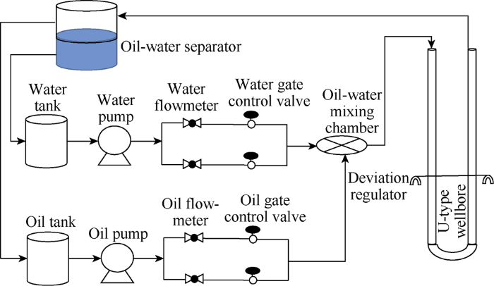
Fig. 1.
Schematics of the setup of multi-phase flow experiment.
1.2. Production logging tool combining micro-capacitance and micro-turbine
The production logging tool for water-oil two phases consists of a micro-capacitance holdup meter and a micro-turbine flowmeter. Its structure is shown in Fig. 2.
Fig. 2.
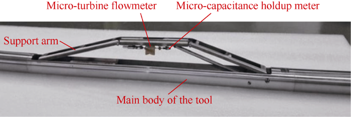
Fig. 2.
Production logging tool for horizontal well.
The micro-turbine flowmeter and the micro-capacitance holdup meter are mounted at the axis with the same height between two support arms to ensure that the flow velocity and phase distribution measured by the production logging tool are at the same position of the cross-section in the test well. The micro-turbine is 28 mm in diameter, the micro-capacitance is 5 mm in diameter, and the main body of the tool is 43 mm in outside diameter. During the experimental tests, the test position of the production logging tool was adjusted by changing the height of the tool arms. The test heights (height from the inner wall at the wellbore bottom) were 48, 64, 76, 88, and 100 mm respectively. When the test at one height was finished, the tool was adjusted to another height to continue measurement. The well flow-section and distribution of test points are shown in Fig. 3.
Fig. 3.
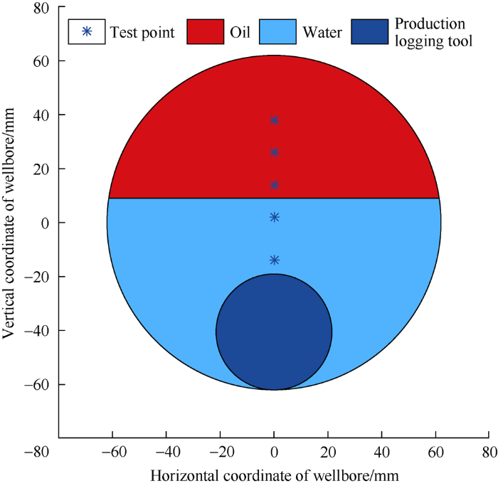
Fig. 3.
Well flow-section and measurement points distribution.
1.3. Responses of micro-turbine flowmeter
Firstly, response characteristics of micro-turbine flowmeter immersed in water and oil respectively were analyzed. It can be seen from Fig. 4 when the turbine was fully immersed in water, at the lowest test point with a height of 48 mm, the turbine did not start at low flow rate, and only started until the total flow reached 120 m3/d, and at the highest test point with a height of 100 mm, the turbine also did not start at the total flow rate of 50 m3/d, and started until the total flow rate reached 70 m3/d, but its response was unstable. At the middle test points with heights of 64, 76, and 88 mm respectively, the turbine started at all total flow rates, and the turbine speed was approximately in linear positive correlation with the total flow rate. When the turbine was fully immersed in oil, at the lowest test point with the height of 48 mm, the turbine started to start until the total flow reached 200 m3/d, and at the highest test point with the height of 100 mm, the turbine did not start at the total flow rate of 50 m3/d only, responded well at the other total flow rates. In this case, the response of the turbine was consistent at the medium height test points, the turbine speed was approximately in linearly positive correlation with the total flow rate. On the whole, the turbine has higher speed when fully immersed in water than fully immersed in oil, this is because that oil is more viscous than water, and at the same condition, when the pipe is filled with oil, the flow rate is more significantly affected by the viscous force against the wall and the tool than with the water.
Fig. 4.
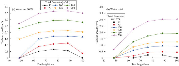
Fig. 4.
Test results of the turbine flowmeter at five test points immersed in oil and water respectively.
Secondly, the response characteristics of the turbine flowmeter at different water cuts were analyzed. It can be seen from Fig. 5 that at the total flow rates of 50 m3/d and 70 m3/d, when the water cut was low, the turbine did not spin at some test points; with the increase of the water cut, the turbine speed at the lower position was generally higher than that at the higher position; at the same total flow rate and water cut, the turbine speed increased with the increase of the test height when the water cut was low (less than or equal to 50%), and it decreased with the increase of the test height when the water cut was greater than 50%. This may be caused by the change of position of maximum local velocity resulted by the rise of the oil-water interface.
Fig. 5.
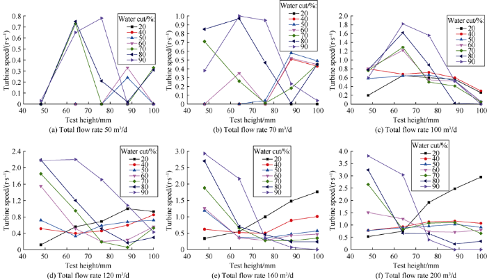
Fig. 5.
Test results of the turbine flowmeter at five test points with different water cuts.
1.4. Responses of micro-capacitance water holdup meter
The response frequency of micro-capacitance water holdup meter is 13 100 Hz when it is immersed in water, and 34 200 Hz when it is immersed in oil. It can be seen from Fig. 6 that the response frequency of the mico-capacitance water holdup meter is obviously correlated with the oil and water distribution. The oil and water show clear stratified flow at low flow rate, the water settling to the bottom with low response frequency and the oil floating in the upper side with high response frequency. At high flow rate, a mixture layer appears at the oil-water interface. With the increase of water cut, the response frequency at higher test position increases gradually with the increase of height. Therefore, the position of the oil-water interface can be determined by measuring the response frequency of the micro-capacitance water holdup meter at the 5 test points across the wellbore.
Fig. 6.
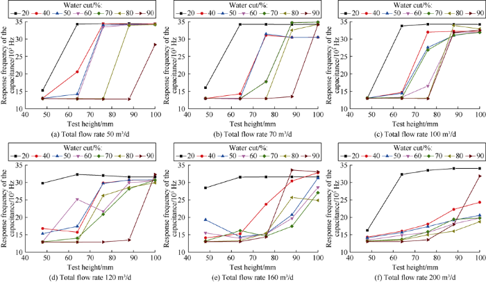
Fig. 6.
Test results of the micro-capacitance water holdup meter at 5 test points with different water cuts.
2. Calculation model of flow rates of different phases in stratified oil-water flow in horizontal well
It can be seen from the experimental data of dynamic measurement of oil-water two phase flow that the frequency responses of the capacitance water holdup meter at 5 test points in the wellbore can be used to determine the oil-water interface height and oil-water distribution of the oil-water stratified flow. Combined with the speed of the turbine at 5 test points, the oil-water velocity field distribution can be worked out, and then the flow rates of the two phases in stratified oil-water flow can be calculated.
2.1. Water holdup calculation model
Based on the water holdup values tested at the five points, the Kriging interpolation algorithm was used to predict the local frequency response at other points on the flow section[9]. The mathematical expression is given as:
The Kriging interpolation algorithm needs to first determine the variogram function of the study area variables. Let Z(x) be the value of a certain property Z of the system at the spatial position x, and Z(x) be a random variable in a region which satisfies the second-order stationary assumption, Z(xq) and Z(xq+h) are the measured values of Z(x) at the spatial positions xq and xq+h, respectively, h is the distance between the two sampling points, and N(h) is the number of sampling points. The discrete calculation equation of the variogram function is expressed as:
The Kriging interpolation algorithm was used to calculate the local water holdup at each test point on the flow section of the wellbore, and the fluid distribution across the section is indicated by pixels of different colors (Fig. 7), and then the height of the oil-water interface was defined based on the image. Due to the design characteristics of the tool, when the oil-water interface is below the upper boundary of the tool, the oil-water interface can’t be measured and the calculated water holdup is distorted.
Fig. 7.
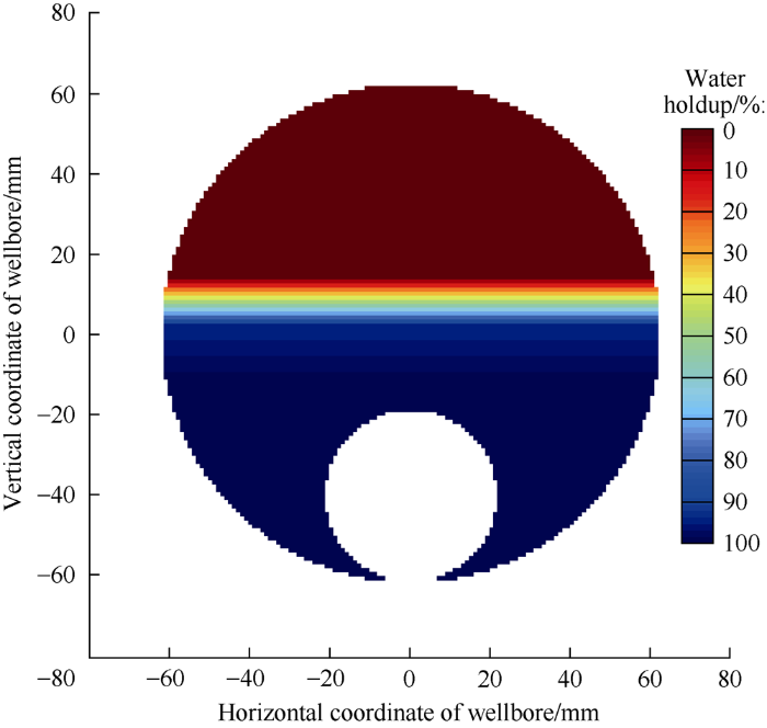
Fig. 7.
Water holdup interpolation image.
2.2. Fluid velocity model
The turbine speed is a linear function of the local fluid velocity, and its response equation is given by[10]:
The conversion coefficient and startup speed of turbine in equation (3) are dependent on the geometric structure and material of the turbine, and properties of the measured fluid.
2.2.1. Numerical simulation of velocity field of the flow section
Based on flow velocity at five test points measured by the micro-turbine, the distribution of fluid velocity over the flow section can be described by the Navier-Stokes equation (N-S equation). In rectangular coordinates, assuming that the fluid flows along the z-axis direction, and the vertical and horizontal directions of the wellbore cross section are the x-axis and y-axis, respectively, then the fluid in the wellbore should satisfy the following equation[11]:
In the pipe, both oil and water meet the continuity equation and momentum conservation equation, so they meet the following boundary and coupling conditions.
Fluid velocity at the inner wall of wellbore is zero:
Fluid velocity at the outer wall of the logging tool is also zero:
At the oil-water interface, the velocities of oil and water of upper and lower layers are single values, in other words, there is no-slip between oil and water[12], that is:
Based on the geometry of the flow section, the physical properties of the fluid, and the height of the oil-water interface, the finite difference was used in equation (4), combined with the boundary and coupling conditions shown in equations (5) to (8), Gauss-Seidel iteration was used to calculate the fluid velocity value at each point on the flow section[13,14]. It can be seen from Fig. 8 to Fig. 10 that when only water phase or oil phase flows, the high value points of the velocity field is mainly distributed at the position between the upper part of the tool and the top of the wellbore; when the oil and water flow in separated layers, the high-value points of velocity field are mainly distributed in the water phase at the upper part of the water phase below the oil-water interface.
Fig. 8.
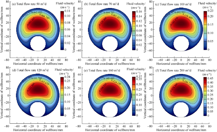
Fig. 8.
Two-dimensional distribution of single-phase water velocity field in horizontal well obtained by numerical simulation.
Fig. 9.

Fig. 9.
Two-dimensional distribution of single-phase oil velocity field in horizontal well obtained by numerical simulation.
Fig. 10.

Fig. 10.
Two-dimensional distribution of velocity field of stratified oil-water flow in horizontal well obtained by numerical simulation (at total flow rate of 50 m3/d and water cut of 50%).
2.2.2. Calculation of fluid velocity at test point
The velocities of the fluid at five test points can be read from Fig. 8 and Fig. 9, and combined with the turbine flowmeter responses at the five test points under the same conditions shown in Fig. 4, the turbine flowmeter response relationships both in water and oil can be obtained, which are shown in Fig. 11 and Fig. 12. Then, combined with equation (3), the conversion coefficient and startup speed of the turbine in single water phase were calculated at 9.138 8 r/m and 0.032 7 m/s respectively, the conversion coefficient and startup speed of turbine in single oil phase were calculated at 7.817 4 r/m and 0.090 9 m/s respectively. This work is equivalent to calibrating the turbine in water and oil to obtain the tool parameters of the turbine in water and oil. In stratified oil-water flow of horizontal well, the fluid nature and the height of the oil-water interface must be determined by the previous water holdup calculation model according to the response frequency of the capacitance sensor, and the corresponding tool parameters are substituted into equation (3) to calculate the fluid velocity at the 5 test points. When the test point is in water, the velocity calculation equation is:
Fig. 11.
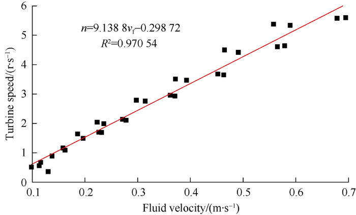
Fig. 11.
Response relation of turbine in single water phase of horizontal well.
Fig. 12.

Fig. 12.
Response relation of turbine in single oil phase of horizontal well.
When the test point is in oil, the equation is
2.3. Calculation model of flow rates of different phases
In order to calculate the flow rate of the fluid in the flow section, the flow section is divided into several mesh grids, and the area of each grid is ΔS, as shown in Fig. 13.
Fig. 13.

Fig. 13.
Meshing diagram of the flow section.
Assuming that there is no slip between the fluid in mesh grids, then the fluid velocity in the micro-grid is equal everywhere:
It can be seen from the numerical simulation of the velocity field of the stratified oil-water two-phase flow that the fluid velocity at any point on the flow section is the function of the position of the point, the height of the oil-water interface, and the turbine speed at the test point:
The fluid velocity of a point obtained by equation (13) is the theoretical value. In actual measurement, the measured fluid velocity can be calculated by using the turbine speed and according to equation (9) and equation (10). Thus, the optimization equations can be given as:
During the finite difference numerical calculation of equation (4), equation (14) is solved with least square method by changing the parameters in the constraint conditions to adjust a set of parameters to be solved, including ni. Fluid velocity at each grid position on the flow section can be obtained, and then it is substituted into equations (11) and (12) to calculate the flow rates of oil and water phases across the flow section respectively.
Taking the total flow rate of 100 m3/d as an example, the two-dimensional distributions of velocity fields on the flow section at different water cuts are shown in Fig. 14, and the results from experimental test and model calculation are shown in Table 1. It can be seen that the measured values and calculated values of the five test points at each water cut are basically consistent. The calculated velocity values of the five test points have an average relative error of 8.308%, and the total flow rates calculated have an average absolute error of 0.457 m3/d, and the calculated water cut values have an average relative error of 2.373%.
Fig. 14.

Fig. 14.
Two-dimensional distributions of velocity fields at different water cuts and the total flow rate of 100 m3/d.
Table 1 Comparison of results from experimental test and model calculation at the total flow rate of 100 m3/d.
| Experimental value | Value calculated by the model | ||||||||
|---|---|---|---|---|---|---|---|---|---|
| Water cut/% | Test height/ mm | Turbine speed/ (r·s-1) | Fluid velocity/ (m·s-1) | Fluid velocity/ (m·s-1) | Relative error of fluid velocity/% | Total flow rate/ (m3·d-1) | Absolute error of the total flow rate/(m3·d-1) | Water cut/% | Relative error of water cut/% |
| 20 | 100 | 0.26 | 0.123 1 | 0.130 1 | 5.35 | 99.01 | 0.99 | 21.32 | 6.60 |
| 88 | 0.56 | 0.148 2 | 0.166 3 | 10.87 | |||||
| 76 | 0.60 | 0.151 6 | 0.184 6 | 17.90 | |||||
| 64 | 0.65 | 0.155 7 | 0.181 6 | 14.24 | |||||
| 48 | 0.20 | 0.118 1 | 0.121 7 | 2.94 | |||||
| 40 | 100 | 0.30 | 0.126 5 | 0.113 8 | 11.14 | 100.22 | 0.22 | 41.57 | 3.93 |
| 88 | 0.60 | 0.151 6 | 0.150 7 | 0.57 | |||||
| 76 | 0.72 | 0.161 6 | 0.176 6 | 8.50 | |||||
| 64 | 0.68 | 0.158 3 | 0.190 2 | 16.80 | |||||
| 48 | 0.80 | 0.120 4 | 0.111 1 | 8.36 | |||||
| 50 | 100 | 0.06 | 0.106 4 | 0.107 1 | 0.64 | 99.71 | 0.29 | 51.49 | 2.98 |
| 88 | 0.53 | 0.145 7 | 0.142 6 | 2.18 | |||||
| 76 | 0.66 | 0.156 6 | 0.168 2 | 6.91 | |||||
| 64 | 0.64 | 0.154 9 | 0.182 7 | 15.21 | |||||
| 48 | 0.58 | 0.096 3 | 0.109 5 | 12.04 | |||||
| 60 | 100 | 0.06 | 0.106 1 | 0.100 8 | 5.24 | 100.18 | 0.18 | 59.35 | 1.08 |
| 88 | 0.52 | 0.144 9 | 0.134 7 | 7.55 | |||||
| 76 | 0.55 | 0.147 4 | 0.159 6 | 7.66 | |||||
| 64 | 1.22 | 0.166 4 | 0.181 5 | 8.35 | |||||
| 48 | 0.81 | 0.121 5 | 0.111 1 | 9.35 | |||||
| 70 | 100 | 0.05 | 0.105 6 | 0.090 3 | 16.92 | 100.19 | 0.19 | 70.26 | 0.37 |
| 88 | 0.41 | 0.135 7 | 0.121 1 | 12.04 | |||||
| 76 | 0.50 | 0.143 2 | 0.144 4 | 0.83 | |||||
| 64 | 1.29 | 0.174 0 | 0.212 6 | 18.15 | |||||
| 48 | 0.76 | 0.116 0 | 0.113 0 | 2.67 | |||||
| 80 | 100 | 0.079 2 | 100.59 | 0.59 | 79.47 | 0.66 | |||
| 88 | 0.02 | 0.103 1 | 0.106 8 | 3.49 | |||||
| 76 | 0.89 | 0.130 2 | 0.140 8 | 7.50 | |||||
| 64 | 1.62 | 0.210 1 | 0.236 6 | 11.19 | |||||
| 48 | 0.78 | 0.118 2 | 0.111 9 | 5.63 | |||||
| 90 | 100 | 0.062 2 | 100.17 | 0.17 | 90.26 | 0.29 | |||
| 88 | 0.52 | 0.089 8 | 0.084 4 | 6.34 | |||||
| 76 | 1.56 | 0.203 6 | 0.213 8 | 4.79 | |||||
| 64 | 1.82 | 0.232 0 | 0.250 9 | 7.53 | |||||
| 48 | 0.60 | 0.098 5 | 0.104 0 | 5.28 | |||||
In order to avoid any misinterpretation due to experimental uncertainties, the calculated and measured water apparent velocities at each test point at the total flow rates of 50, 70 and 100 m3/d were compared. It can be seen from Fig. 15 that they agree well.
Fig. 15.
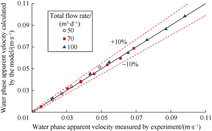
Fig. 15.
Comparison of the calculated and measured water apparent velocities in the horizontal well.
3. Conclusions
The simultaneous measurement mode of micro-capacitance and micro-turbine at the same height was adopted to get their responses at the same measuring height, which has improved the accuracy of local fluid identification and flow rate measurement.
Since the turbine flowmeter has a startup speed threshold, at low flow rates, the turbine didn’t spin or was unstable in response at the lowest test point near the tool body and at the higher test point near the top wall of the wellbore. In contrast, at moderate to high flow rates, the turbine flowmeter response value had a linear relationship with the fluid flow velocity, and the turbine had high response efficiency. The response frequency of the capacitance water holdup meter is obviously related to the oil-water distribution at its position, which reflects the stratified state of the oil and water well. When the oil-water interface is located above the upper boundary of the tool body, the height of the oil-water interface can be determined by the water holdup interpolation imaging map, and then it can be further used in numerical simulation of the velocity field of the flow section.
Based on the local velocity values at five test points picked up from the two-dimensional distribution map of the velocity field of the flow section obtained by numerical simulation, an objective function was established to minimize the deviation between the calculated velocity and measured velocity, then a optimization method was used to calculate velocity field of the stratified oil-water two-phase flow in the horizontal well, so as to calculate the flow rate of each phase. The calculated velocities and measured velocities at the five test points are basically consistent, and the calculated total flow rates and water cuts are basically consistent with those set in the experiments, which prove the method presented in this paper can work out flow rates of different phases in stratified oil-water flow in horizontal well at total flow rates of more than 50 m3/d and water cuts from 20% to 90%.
Nomenclature
ci—reliability coefficient of measurement data by micro-turbine flowmeter at the ith test point;
g—gravitational acceleration, 9.8 m/s2;
gi(X)—objective constraint function containing unsolved parameters including vfc,i;
hw—height of the oil-water interface, m;
i—serial number of the test point;
j—serial number of non-test point;
k—serial number of cross-section mesh;
K—conversion coefficient of turbine, r/m;
n—turbine speed, r/s;
pz—pressure in the direction of fluid flow, Pa;
Qo, Qw—oil, water flow rate, m3/s;
r—tool outside radius, m;
R—wellbore inner radius, m;
Ti—water holdup tested at the ith point , %;
Tj—predicted water holdup at the jth non-test point, %;
vf—fluid velocity, m/s;
vfc,i—calculated fluid velocity at the ith point, m/s;
vfe,i—measured fluid velocity at the ith point, m/s;
vo, vw—oil and water velocities, m/s;
vth—turbine startup speed, m/s;
x, y, z—rectangular coordinate system, m;
X—vector containing the unsolved parameters including vfc,i;
ΔS—area of one mesh grid, m2;
γ(xi,xj)—variogram function between test point and non- test point;
θ—deviation angle, (°) ;
μ—fluid viscosity, Pa·s;
μo, μw—oil and water viscosities, Pa·s;
ρ—fluid density, kg/m3.
Reference
The analysis and modelling of measuring data acquired by using combination production logging tool in horizontal simulation well
Gas-water phase flow production stratified logging technology of coalbed methane wells
A study of oil/water flow patterns in horizontal pipes
An experimental study of oil water flows in horizontal pipes
Oil water flow pattern transition prediction in horizontal pipes
DOI:10.1115/1.4031608 URL [Cited within: 1]
Production logging low flow rate wells with high water cut
Liquid-liquid horizontal pipe flow: A review
Analysis on imaging interpolation algorithm for logging data of water holdup array tool in horizontal wells
Mathematical model on stratified laminar flow in pipe
Numerical simulation of velocity fields of oil-water stratified flows in horizontal wells
Analysis of stratified oil-water two-phase flow between inclined parallel plates
Numerical simulation of solid-liquid two-phase steady flow in horizontal pipe
