


Introduction
Seismic inversion technology has made great progress in the past 40 years. Experts and scholars, such as Zhao[1], Yin[2], Sa[3] and Gan[4], systematically summarized the development status of seismic inversion technology. At present, seismic inversion technologies widely used in petroleum industry mainly include three kinds: the first kind is geophysical inversion based on convolution model[5], which has evolved from post-stack "bright spot" technology to wave impedance inversion technology[6], prestack AVO technology[7], and elastic wave impedance inversion technology[8]. In recent years, with the development of wide azimuth seismic technology, the seismic inversion has further expanded to OVT (Offset Vector Tile) domain[9]. The second kind is nonlinear inversion technology, including neural network, support vector machine, Bayesian, pattern recognition and genetic algorithm[3]. The third kind is geostatistical inversion, which improves vertical resolution through random simulation[10].
The above inversion techniques have achieved good results in the field of reservoir prediction, but different in methods and principles, they all have certain limitations. Geophysical inversion based on convolution model cannot break the limitation of seismic resolution[11]. The solutions obtained by nonlinear inversion are often not globally optimal, and the inversion results from this inversion often show poor geological regularity[12]. With high-frequency components coming from stochastic simulation, geostatistical inversion has results with strong randomness and low lateral resolution[13].
The continental sedimentary reservoirs in China have thin thickness and fast lateral variation[14]. At present, the demand for reservoir identification accuracy has reached about 1 m[15], and the existing seismic inversion technologies cannot meet this accuracy requirement. Based on detailed analysis of the internal relationship between seismic waveform and logging high-frequency information, this paper systematically elucidates the principle of seismic meme inversion. In this inversion, lateral similarity of seismic waveform is used to drive logging high-frequency information to realize high-resolution inversion. Through model validation and example of thin interbed identification in Daqing placanticline, it is concluded that seismic meme inversion can better solve the prediction problem of sand body in continental thin interbeds.
1. Theoretical basis of seismic meme inversion method
1.1. Discussion on seismic vertical resolution and lateral resolution
Seismic resolution is divided into vertical resolution and lateral resolution. The concept of vertical resolution first proposed by Rayleigh[16] is that the resolution limit of two adjacent reflection interfaces is 1/4 wavelength, and geological bodies with thickness less than 1/4 wavelength can be defined as thin layers and cannot be distinguished by seismic data. In order to solve the problem of thin reservoir prediction, many researches have been carried out. Wides[17] proposed that under ideal conditions, thin layers with arbitrary thickness could be identified according to lateral amplitude variations. Zeng[18] advanced the concept of "lateral detection rate", and that stratal slice can be used to detect lateral changes of geological bodies with thickness less than 1/4 wavelength.
Here, the vertical resolution and lateral resolution of thin layer were discussed by a forward model. The geological model was designed to contain a 3 m thick sandstone layer in continuous distribution, a set of lenticular thin sandstone layer 0-3 m thick above the sandstone layer (Fig. 1a), and a mudstone interlayer 3 m thick between them under the background of mudstone. The seismic wave velocities of sandstone and mudstone were supposed to be 3500 m/s and 2800 m/s, and the densities of 2.65 g/cm3 and 2.26 g/cm3, respectively. The convolution was performed by using 35 Hz zero-facies Ricker wavelet. It can be seen from the forward modeling profile (Fig. 1b) that the overlying thin sandstone layer cannot be directly distinguished vertically. But due to the development of the thin sandstone layer, the seismic waveform has changed laterally. By extracting the amplitude and frequency at the maximum peak in Fig. 1b (Fig. 1c), it can be seen that the seismic amplitude and frequency have changed greatly horizontally, that means the seismic waveform contains information of the thin layer. It can be concluded that although the thin layer cannot be "distinguished" by the seismic amplitude in the longitudinal direction, it can be "identified" by the lateral waveform change.
Fig. 1.
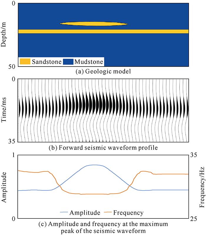
Fig. 1.
The geological model and forward modeling profile.
1.2. Internal relationship between seismic waveform and logging high-frequency information
Seismic waveform contains information of seismic kinematics and dynamics, which is the comprehensive response of geological information such as geological sedimentation, lithology and lithofacies combination, reservoir physical properties and fluid. Zeng[19] put forward the concept of "seismic sedimentology", which makes full use of the lateral high resolution of seismic data to improve the prediction accuracy of thin layers, and has been widely used in the prediction of thin reservoirs.
We tried to introduce logging data into seismic sedimentology, and organically combine the horizontal high-resolution of seismic data with the vertical high-resolution of logging curve. The first problem to be solved was how to establish the internal relationship between seismic waveform and high-frequency logging information.
In actual data, similar sedimentary characteristics often accompany similar lithologic association, and similar lithologic association often results in similar seismic waveform charac-teristics. The actual data of a continental thin reservoir was selected for analysis. Fig. 2a shows the seismic profile of wells A and B, the seismic data has high signal-to-noise ratio but low frequency, with the main frequency of about 20 Hz and the frequency width of about 10-35 Hz. The uphole trace seismic waveforms of two wells in the same interval were extracted. Due to the difference in depth between the two wells, the seismic waveforms of the two wells were firstly aligned with the top surface and corrected for thickness consistency, and then superimposed and compared (Fig. 2b). It can be seen from the figure that the correlation coefficient between the waveforms of the two wells reaches 94%. Therefore, the uphole traces of the two wells have similar seismic waveforms.
Fig. 2.
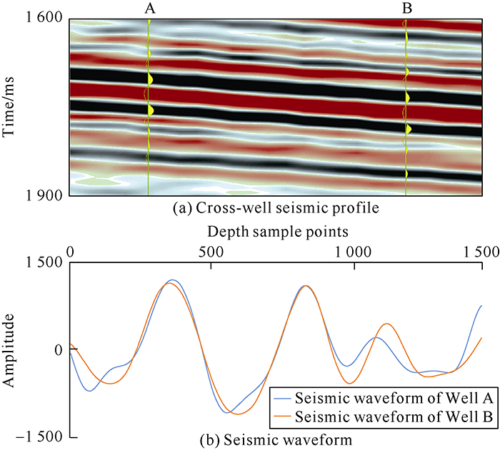
Fig. 2.
Seismic waveforms of wells A and B.
Then the similarity characteristics of the logging curves were examined. Firstly, the P-wave impedance curve directly related to seismic reflection was checked. The correlation coefficient of the original P-wave impedance curves of the two wells is 75% (Fig. 3a), which is much lower than the similarity of their seismic waveforms. This is because the logging curve has very high frequency, and the difference in high-frequency components reduces their similarity. The logging curves were filtered in sequence to preserve the 0-500 Hz, 0-400 Hz, 0-300 Hz, 0-200 Hz and 0-100 Hz signals respectively (Fig. 3b-3f), and the correlation coefficients gradually increased to 88%, 92%, 93%, 94% and 95%, implying very high similarities. It can be seen that due to the difference in high-frequency information, the original logging curve have low similarity. When the high frequency components are filtered step by step, the logging curves increase in similarity gradually. When the frequency of logging curves reaches 200-300 Hz, the correlation coefficient of the logging curves reaches the similarity of seismic waveforms. Therefore, the relationship between seismic waveforms and high-frequency logging information can be established, which provides a basis for high-resolution seismic inversion. When seismic meme inversion is carried out, the optimal cut-off frequency of inversion can be determined by analyzing the similarity of logging curves at different frequencies and the thickness of target reservoir.
Fig. 3.
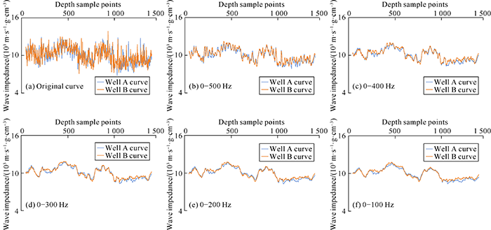
Fig. 3.
Filtering of P-wave impedance curves of wells A and B in different frequency bands.
When the reservoir characteristics are complex and the P-wave impedance cannot distinguish the lithology, log curves such as natural gamma are needed, but seismic inversion based on convolution model cannot predict natural gamma curve. The natural gamma curve was analyzed by the similar way used to analyze the P-wave impedance curves. As shown in Fig. 4a, the correlation coefficient of the original natural gamma curves of the two wells is only 71%, and the natural gamma curves were filtered successively to reserve the frequency components of 0-500 Hz, 0-400 Hz, 0-300 Hz, 0-200 Hz and 0-100 Hz (Fig. 4b-4f). The correlation coefficients gradually increased to 88%, 90%, 92%, 93% and 95%, basically consistent with that of the longitudinal wave impedance curves.
Fig. 4.
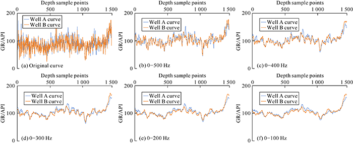
Fig. 4.
Filtering of natural gamma curves of wells A and B in different frequency bands.
From the perspective of sedimentology, within the isochronous stratigraphic framework, the change in seismic waveform reflects the change of lithologic association which is the manifestation of sedimentary facies or seismic facies. From the perspective of logging curve, wave impedance and natural gamma curves etc. all can reflect the changes of lithologic association or sedimentary facies. Therefore, the corresponding relationship between low-frequency seismic information and high-frequency logging information is not only applicable to wave impedance curve, but also to non-wave impedance curves such as natural gamma, which lays the foundation for high-resolution inversion (or simulation) using low-frequency seismic data and high-frequency logging data. It should be noted that wave impedance curve can be used for seismic meme inversion, and the non-wave impedance curves such as natural gamma can be used for seismic meme simulation.
2. Seismic meme inversion
The above analysis of seismic waveforms and logging curves of actual data shows that the logging curves corresponding to similar waveforms show high similarity in a wide frequency band. Therefore, high-resolution inversion can be realized by using the lateral similarity of seismic waveforms to drive high-frequency logging information[20], this is named the seismic meme inversion (SMI) method. The meaning of "meme" is defined in Oxford English dictionary as transmitting information through imitation, that is, by imitating similar seismic waveforms, the high-frequency logging curve information represented by seismic waveform is transmitted to realize high-resolution inversion.
In the process of seismic meme inversion, firstly, the efficient dynamic clustering analysis of seismic waveforms of uphole trace is realized by singular value decomposition, the mapping relationship between seismic waveform structure and logging curve structure is established, and logging curve sample sets of different types of waveform structures (representing different types of seismic facies) are generated. Secondly, the distribution of sample sets corresponding to different types of waveform structures is analyzed, and the Bayesian inversion frames for different types of seismic facies are established; under the different Bayesian frames, the common parts of the sample sets are selected as the initial model for iterative inversion. Finally, in the iterative inversion process, the best cut-off frequency of the sample set is taken as the constraint condition to obtain the high-resolution inversion results. The basic principles of seismic meme inversion mainly include the following three aspects.
2.1. Seismic waveform clustering through singular value decomposition
The corresponding relationship between seismic waveform parameters and well point attributes can be defined as an n×m-order matrix A
where, U and V are seismic waveform data and well point attribute data, which are n×n-order and m×m-order orthogonal matrices respectively, VT is the conjugate transposition of V, and $\Lambda \;$ is the n×m-order non-negative real diagonal matrix, indicating the correlation between seismic waveform data and well point data.
Singular value decomposition is the orthogonal decomposition of A. When the rank of the matrix is r, the matrix A can be decomposed into the algebraic sum of r eigenvectors, and the total energy of matrix A can be expressed as:
After the singular value decomposition of the matrix A through equation (2), the main characteristics of the matrix A can be represented by the singular vectors corresponding to the first r non-zero singular values, that is, to realize the dynamic clustering analysis of seismic waveform, to obtain the corresponding relationship between seismic waveforms and logging curves of different reservoir types, and to establish the initial sample set.
2.2. Wavelet transform of logging curve
Wavelet transform converts the digital signal from time domain to frequency domain, which can describe the signal characteristics in time domain and frequency domain, and can quantitatively predict low-frequency stable part and high-frequency mutation part of signal.
For the logging curves of the sample set established in Section 2.1, formula (3) was used to carry out discrete wavelet transform at different cut-off frequencies to decompose the logging curve into three parts: low-medium frequency macroscopic characteristic information, high frequency detail information and ultra-high frequency noise information. It should be noted that since the logging curves have very high frequencies, taking the AC curve as an example, its frequency is as high as 20 kHz[21], therefore, the low-medium frequency defined here is about 100-200 Hz, even 300-400 Hz, that is, "logging high-frequency information" defined in this paper relative to the seismic frequency range. The extracted low-medium frequency macroscopic characteristic information is the common structure of all logging curves in the sample set, which can be used as the initial model of seismic meme inversion.
2.3. Seismic meme inversion in Bayesian framework
The basis of seismic inversion is convolution model:
Suppose that noise n satisfies Gaussian distribution
By substituting equation (5) into equation (4), the likelihood function of seismic data is established
In Bayesian inversion, assuming that the elastic parameter model m also conforms to Gaussian distribution, the priori distribution of the model can be obtained as follows:
The product of data conditional probability distribution and model prior probability distribution is taken as the posterior probability distribution function of the model:
For a given seismic waveform d, the expected value of model m can be calculated by using Gibbs sampling method according to the posterior probability.
In equation (8), the solution obtained at the maximum probability is the final solution of inversion. The logarithm of the two ends of equation (8) is obtained:
In order to maximize the posterior probability, the derivation of equation (8) with respect to the model parameter Δm is calculated to obtain the objective function:
Let $O'\left( {\Delta {\bf{m}}} \right)$ =0, then the model disturbance quantity is:
The iterative model perturbation method is used to approximate the sample data to get the final high-resolution inversion results.
The seismic meme inversion method has the following characteristics:
(1) Seismic meme inversion uses the lateral variation of seismic waveform to drive high-frequency logging information to realize high-resolution inversion. The inversion results are in consistent with the high frequency information of logging vertically, and have high vertical resolution (when the common structure of high frequency of logging curve is 200-300 Hz, the resolution of thin layer prediction is 2-3 m). At the same time, the inversion results follow the changes of seismic waveform horizontally, and also have high horizontal resolution. Therefore, seismic meme inversion can simultaneously improve the vertical and horizontal resolution of inversion results, and is indeed a high-precision inversion method.
(2) The only available data between wells is seismic data. The lateral variation of seismic waveform reflects the change in lithofacies combination and seismic facies. The seismic meme inversion realizes the inversion under the automatic control of seismic facies by replacing the interpolation simulation of variogram spatial domain with lateral variation of seismic waveform. This method overcomes the subjectivity caused by the traditional facies-controlled inversion which needs to set the sedimentary facies manually in advance, so it is facies controlled inversion in the real sense.
(3) Seismic meme inversion method not only realizes high-resolution wave impedance inversion, but also realizes facies-controlled high-resolution simulation of non-wave impedance parameters such as natural gamma, resistivity and porosity logs. It breaks the limitation that seismic inversion can only obtain wave impedance results. It is a great progress for reservoir parameter simulation using seismic information.
3. Validation of the method
In order to verify the rationality of the meme inversion method and its ability to recognize thin interbeds, a forward model of thin interbeds was established to do inversion experiments.
The geological model is as follows (Fig. 5): it had four groups of thin interbedded sand bodies in the mudstone background. The first group was composed of three sandstone layers of 3 m thick each, and the mudstone interlayers were 3 m thick each too. One of the sandstone layers was removed in the next three groups. The velocities of the sandstone and mudstone are 3500 m/s and 2800 m/s respectively, and the densities were 2.65 g/cm3 and 2.26 g/cm3, respectively. In order to facilitate seismic meme inversion, nine virtual wells (W1-W9) were established on the model to represent characteristics of different reservoirs.
Fig. 5.
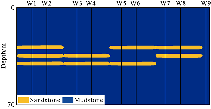
Fig. 5.
Thin interbed geological model.
The geological model was convoluted by using zero-facies Ricker wavelets with a dominant frequency of 30 Hz to 120 Hz, and the seismic forward profiles with dominant frequencies of 30, 60 and 120 Hz representing low frequency, medium frequency and high frequency were selected to carry out different inversion experiments. Fig. 6a to 6c shows seismic forward modeling profiles at dominant frequencies of 30, 60 and 120 Hz respectively, and the yellow curves are P-wave impedance curves. It can be seen from the figure that due to the low resolution, the 30 Hz seismic data can’t identify the thin interbedded sand bodies at all, but due to different sand body combinations, showing big differences in the seismic waveforms. The 60 Hz seismic data can only identify the third group of sandbodies, and the 120 Hz seismic data can identify each thin sandbody of the four groups.
Fig. 6.
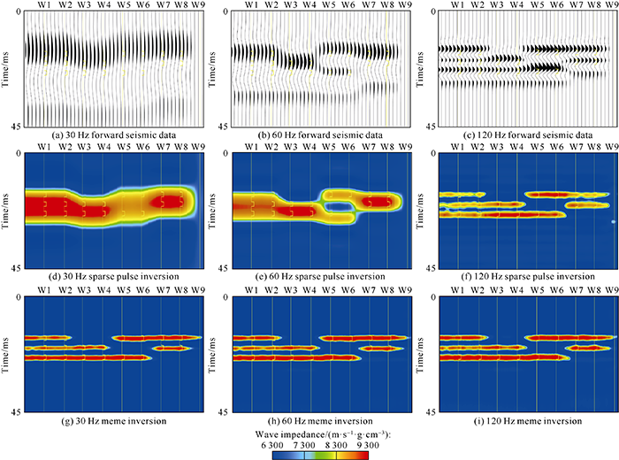
Fig. 6.
Forward modeling seismic data with different dominant frequencies and inversion profiles by different methods.
First, conventional sparse pulse inversion was carried out using forward seismic data. Fig. 6d to 6f shows sparse pulse inversion profiles with dominant frequencies of 30 Hz, 60 Hz and 120 Hz, respectively. It can be seen from the figure that the resolution of sparse pulse inversion is similar to that of seismic data. The 30 Hz inversion results cannot identify thin interbedded sand bodies at all, the 60 Hz inversion results can distinguish two sandbodies of the third group of sandbodies, the 120 Hz inversion results can distinguish each single sandbody of the four groups of sandbodies.
Then, forward modeling seismic data was used to carry out seismic meme inversion. Fig. 6g to 6i shows the meme inversion results with dominant frequencies of 30, 60 and 120 Hz respectively. It can be seen from the figure that the three results are basically the same in resolution, and all of them can identify each single sand body of the four groups of sand bodies.
In order to further verify the noise resistance of seismic meme inversion, 5%, 10% and 20% random noises were added to the seismic trace with dominant frequency of 30 Hz in Fig. 6a (Fig. 7a-7c), and then seismic meme inversion was carried out respectively. From the obtained P-wave impedance results (Fig. 7d-7f), it can be seen that under three different noise levels, all the inversion results can accurately identify 3 m thin sandstone reservoirs. Only in the mudstone background, different degrees of noise appear, but this does not affect the accurate identification of the target sandstone layers, which confirms that the seismic meme inversion method has strong noise resistance.
Fig. 7.
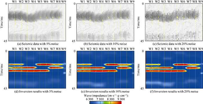
Fig. 7.
30 Hz forward modeling seismic data and seismic meme inversion profiles with random noise of 30 Hz added.
The model validation results show that sparse pulse inversion can’t identify the thin interbedded sand bodies with thickness less than 1/4 wavelength. Seismic meme inversion can break the limit of 1/4 wavelength. As long as the seismic waveforms have horizontal differences, it can identify thin interbedded sandbodies even in the case of low resolution of seismic data. At the same time, random noise inversion test results show that the seismic meme inversion has strong noise resistance.
4. Application examples
4.1. Reservoir characteristics
The study area is located in Putaohua reservoir of Cretaceous Yaojia Formation in the north of Daqing placanticline in the Songliao Basin. Previous studies show that controlled by the northern water system, the northern area of Daqing placanticline had a large river-delta complex, and nearly north-south underwater distributary channel deposits widely developed in stratigraphic sedimentary period[22]. The sand bodies are 900-1200 m deep and 0.2-15.0 m thick each, and 47% of the sand bodies are 1-3 m thick (Fig. 8a), showing typical characteristic of thin interbedding. In the late stage of oilfield development, the main target layers to tap remaining oil have changed from thick sand bodies to sand bodies with small thickness and fast lateral change, so it is necessary to finely characterize the thin interbedded sand bodies.
Fig. 8.
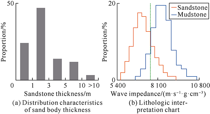
Fig. 8.
Sand body thickness and lithologic interpretation chart.
Lithologic logging interpretation was carried out by using well logging and mud logging data, and sand-mud interpretation chart was established (Fig. 8b). The P-wave impedance of sandstone is less than 7600 m·g/(s·cm3). Therefore, the P-wave impedance can be used to identify sandstone and mudstone, and seismic meme inversion can be carried out to obtain P-wave impedance results to predict sandstone distribution.
4.2. Application of seismic meme inversion
The area of seismic 3D work area in this study is 6.25 km2, and there are 39 wells drilled in relatively uniform distribution in the work area. In order to verify the rationality of meme inversion algorithm, different numbers of wells were used in the inversion: in the first group, all the 39 wells participated in the inversion (Fig. 9a, 9b); in the second group, 10 wells were randomly selected from the 39 wells to participate in inversion, and the remaining 29 wells were verification wells (Fig. 9c, 9d); in the third group of experiment, simulating and evaluating the uneven well pattern, 25 wells in the north participated in inversion, and 14 wells in the south were verification wells (Fig. 9e, 9f). From the inversion profiles of the above three groups of experiments (Fig. 9a, 9c, 9e), it can be seen that the inversion results of both participating wells and verification wells show high consistency with the drilling data, and the inversion results of the three groups of experiments are highly similar. According to the threshold value of sandstone determined by lithology histogram, the thickness maps of sandstone in the upper oil layer group (black dotted frame in inversion section, Fig. 9a, 9c, 9e) were extracted (Fig. 9b, 9d, 9f). It can be seen from the figure that the shapes of the three thickness maps are basically the same, showing two branches of channel sandbodies in nearly north-south direction, clear boundary of the main channel, and channel distribution conforming to the geological law.
Fig. 9.

Fig. 9.
Comparison of results of inversions with different numbers of participating wells.
In order to further quantitatively describe the accuracy of the inversion prediction, the sand body thickness of the upper oil layer group predicted by inversion was extracted and compared with that interpreted from logging. Fig. 10a shows the comparison of results from the inversion with all 39 wells participating with the thickness from logging interpretation, and the correlation coefficient between sandstone thickness predicted by the inversion and sandstone thickness from logging interpretation is 90.8%. Fig. 10b shows the comparison of sandstone thickness from the inversion with 10 wells randomly selected in the simulation exploration stage, the red spots are the wells participating the inversion, the sandstone thickness of these wells from the inversion has a correlation coefficient of 91.2% with that from logging interpretation; and the blue points are the sandstone thickness of verification wells, which has a correlation coefficient of 80% with that from logging interpretation. Fig. 10c shows the comparison of sandstone thickness from the inversion with 25 wells in the north participating in the evaluation stage. The red spots indicate the sandstone thickness of wells participating the inversion, which has a correlation coefficient of 90.2% with that from logging interpretation; and the blue spots indicate the sandstone thickness of the verification wells from the inversion, which has a correlation coefficient of 80.8% with that from logging interpretation.
Fig. 10.

Fig. 10.
Cross plot of sandstone thickness predicted by inversion and sandstone thickness interpreted from the logging data.
Through the comparison of inversion results of different methods mentioned above and with different numbers of wells, it can be seen that the meme inversion results have two advantages: (1) The meme inversion has high resolution, can identify thin interbeds 2-3 m thick, and has high inversion accuracy, with a 90% coincidence rate of participating wells, and 80% coincidence rate of verification wells. (2) In the meme inversion, the seismic waveform drives the logging curve to realize high-resolution inversion, which has the idea of facies control, and is not affected by the number of wells and the distribution of well locations, and the inversion results conform to the geological laws.
4.3. Comparison of different inversion methods
The results of seismic meme inversion have an identification accuracy of 2 m for the thin interbeds in the Daqing placanticline. By comparing the results of seismic meme inversion and the main stream deterministic inversion method, sparse pulse inversion, it is further proved that the seismic meme inversion has higher accuracy.
The target layer has a main frequency of 40 Hz on the 3D seismic data, and the longitudinal wave velocity is about 3000 m/s. According to the theory of 1/4 wavelength of seismic resolution, the maximum thickness that can be identified by the seismic data is about 18.75 m, which obviously does not meet the requirements of identifying thin interbedded sandbodies. It can be seen from the seismic profile passing through wells (Fig. 11a) that the seismic data can’t identify thin interbedded sand bodies of Putaohua reservoir. First, conventional sparse pulse inversion was carried out. From the obtained P-wave impedance profile (Fig. 11b), it can be clearly seen that the results of sparse pulse inversion are roughly the same in resolution as seismic data, and can only roughly indicate the large sets of sandstone, but cannot predict thin interbedded sand bodies. Then, seismic meme inversion was carried out. From the obtained P-wave impedance inversion profile (Fig. 11c), it can be seen that the longitudinal resolution of meme inversion results is obviously higher than that of sparse pulse inversion results, and can indicate thin interbedded sandbodies. Meanwhile, the lateral variation characteristics of sandstone in the seismic meme inversion results conform to seismic characteristics, and can better describe the lateral boundary of the sand bodies, that is, meme inversion also has high lateral resolution.
Fig. 11.

Fig. 11.
Comparison of a seismic profile with inversion profiles from different methods.
In order to further quantitatively demonstrate the accuracy of the two inversion methods, the curves at well points were extracted from the two inversion data volumes (taking well W3 in Fig. 11 as an example). The first and second red curves in Fig. 12 are measured P-wave impedance curves (for comparison with inversion results, the actual P-wave impedance curve was filtered at a sampling rate of 2 m). It can be seen that the meme inversion result is much more consistent with the measured curve than the sparse pulse inversion result. The lithology of the results from the two kinds of inversion was interpreted according to the sandstone threshold value. Compared with the lithologic interpretation results from actual logging data (Fig. 12), the interpreted lithology from meme inversion is in better agreement with the lithology from logging interpretation, with sandstone layers 1.8-3.0 m thick identified; while the lithology interpreted from sparse pulse inversion results is in low agreement with the lithology from logging interpretation, with sand bodies 10 m thick identifiable. Apparently, seismic meme inversion results have much higher coincidence rate and accuracy than sparse pulse inversion results.
Fig. 12.
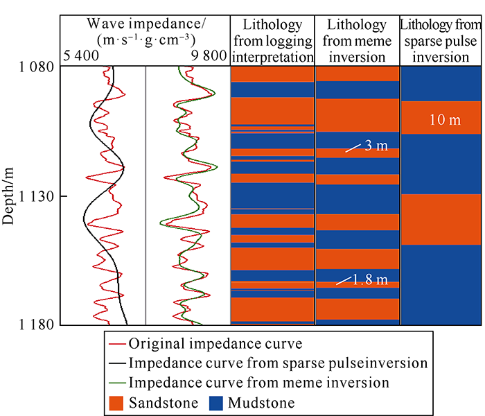
Fig. 12.
Comparison of results from sparse pulse inversion and waveform indication inversion.
5. Conclusions
Seismic meme inversion establishes the mapping relationship between seismic waveform structure and high-frequency logging curve structure through dynamic clustering of seismic waveform, and improves the vertical and horizontal resolution of inversion results. By constructing Bayesian inversion framework of different seismic facies types, this inversion method can realize facies-controlled inversion in the real sense.
The model verification results of seismic meme inversion and its application in Daqing placanticline show that the seismic meme inversion results could reach the recognition accuracy of 2 m, and the coincidence rate of inversion results and drilling wells was more than 80%. Seismic meme inversion can improve the accuracy of reservoir prediction, and provide a reference for the identification of thin interbedded sandstone layers with fast lateral facies change in continental basins.
Its application in Daqing placanticline shows that seismic meme inversion is suitable for exploration, evaluation and development stages. But the basic principle of this method requires that the drilled wells cover all the main sedimentary facies types in the study area as much as possible. Therefore, a certain number of drilled wells are needed in its practical application, so it is not suitable for the early stage of exploration with few wells drilled. Seismic meme inversion is also applicable to carbonate and volcanic reservoirs. When carbonate and volcanic reservoirs are layered media, the requirements and precautions for this inversion are the same as those for clastic reservoirs. When carbonate or volcanic reservoirs are hilly media, a framework model of the mound media must be constructed through fine horizon interpretation to obtain ideal inversion result.
Nomenclature
A—matrixes of seismic waveform data and well point attribute data;
U—seismic waveform data matrix;
V—well point attribute data matrix;
$\Lambda \;$—correlation matrixes of seismic waveform data and well point attribute data;
δi—non-negative square root of eigenvalue of AAT;
r—rank of matrix;
l—correlation cut-off frequency of common structure of logging curve, Hz;
W—logging curves of sample wells;
$\overline {\bf{W}}$—average value of logging curves of sample wells;
$\psi (\omega ,t)$—wavelet function;
d—seismic data matrix;
G—seismic wavelet matrix;
m—matrix of elastic parameter model to be solved;
n—noise matrix;
N—number of sample sets;
I—priori information matrix;
σ—covariance of seismic data;
σm—model variance;
Δm—disturbance quantity of model parameters;
σΔm—disturbance variance of model parameters;
R—correlation coefficient between sand body thickness predicted by inversion and sandstone thickness from log interpretation, %;
GR—natural gamma curve, API.
Reference
Research progress of fluid discrimination with pre-stack seismic inversion
Past, present, and future of geophysical inversion
Current status and development trends of seismic reservoir prediction viewed from the exploration industry
Evolution of seismic interpretation during the last three decades
Autoregressive recovery of the acoustic impedance
Plane-wave reflection coefficients for gas sands at nonnormal angles of incidence
Research status and progress of 5D seismic data interpretation in OVT domain
Geostatistical inversion: A sequential method of stochastic reservoir modelling constrained by seismic data
Limitations of deterministic and advantages of stochastic seismic inversion
Addition and comparison of nonlinear seismic inversion methods
Predicting method by the well and seismic integration for the fluvial facies reservoirs in Lamadian
Seismic reservoir prediction method for different types of sedimentary sand bodies in terrestrial fault depression
The status and development direction of reservoir geophysics in CNPC
Guidelines for seismic sedimentologic study in non-marine postrift basins
Seismic sedimentology in China: A rview
Application of seismic meme inversion in thin sand distribution prediction under coal shield
A review of study on relation between well logging data and seismic attributes
High-resolution sequence stratigraphy division of Upper Putaohua reservoir, northern Daqing Placanticline
