


Introduction
The accurate prediction of geological features (lithology, formation dip, fracture-cavity, fault, etc.) and the description of drilling geological environment factors (rock drillability, basic data for rate of penetration (ROP) modelling, rock mechanical parameters, formation pressure, etc.) are of great significance in scientific drilling design and efficient drilling operation[1,2]. Over the past years, many scholars and engineers in this field have done extensive studies[3-8] and come up with some systematic theories and methods. Among them, the most common prediction methods are those used before drilling operation which mainly depends on seismic data and offset wells data. However, numerous drilling cases have proved that the accuracy of pre-drilling prediction and description is relatively low due to extrapolating errors from offset well data to the designed well, non-uniqueness problems in seismic velocity model building and subsequent seismic imaging errors[9]. During drilling operation, geological features and drilling geological environment factors of drilled formations can be updated, while those of the formation ahead of bit cannot.
To solve this problem, a seismic guided drilling technology (SGD) has been developed by the well-known service company Schlumberger. In this technology, VSP-while-drilling tool is used to obtain real-time one-dimensional seismic velocity data as constraints to build the well constrained seismic velocity model and reprocess the pre-stack seismic data in a small range around the well, so as to realize the prediction of some geological features and pore pressure of formation ahead of bit while drilling[10]. This technology can greatly improve the prediction accuracy and has played a role in guiding the drilling operation in deep-sea areas of the Gulf of Mexico[11]. Meanwhile, it has been applied in an oilfield of China to optimize the well trajectory control and improved the encountering ratio of carbonate reservoirs[12,13]. However, this technology must be accompanied with the expensive VSP tool and other costly monitoring while drilling (MWD) instruments. Due to low oil price, it has not been widely used in the industry.
To achieve the objectives of safe, high-quality, high-efficiency and low-cost drilling, we propose a new technique considering the situation in China. In this technique, a new real time seismic velocity updating while drilling method under the constraints of conventional wire-logging and mud- logging data measured in drilling process has been established. Based on the updated seismic velocity, the depth migration of seismic data in a small range around the well is conducted to predict and describe some geological features and drilling geological environment factors of certain section ahead of the bit. This technique can extend the scope and improve the accuracy of prediction and description of geological features and drilling geological environment factors. In other words, it can provide more comprehensive forward-looking information for the real-time optimization of drilling decisions.
1. Methodology and workflow
The specific work flow of well-seismic information integration guided drilling technique is as follows (Fig. 1):
Fig. 1.
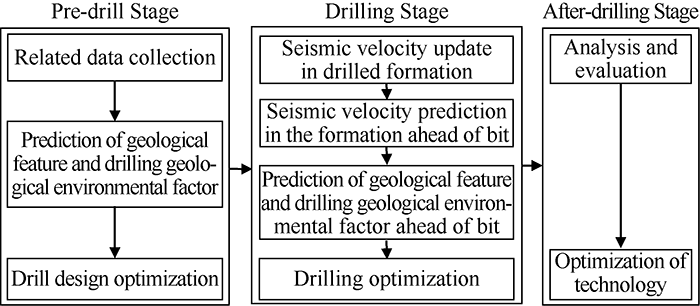
Fig. 1.
The overall workflow of well-seismic integration guided drilling.
(1) Pre-drilling stage. Centered on the designed well location, the pre-stack CMP seismic gather data in a small range around the well (generally the bottom hole displacement plus 3000-5000 m) and the geology, drilling, logging and mud data from offset wells need to be collected. The seismic data and offset well data are processed to realize the preliminary prediction and description of geological features and drilling geological environment factors. The possible obstacles and risks during the upcoming drilling operation are analyzed. Accordingly the drilling program and drilling design are optimized.
(2) Drilling stage. During drilling process, measurements in drilled formation is made in real time (mainly including conventional well logging and geological horizon data, it would be better if the logging while drilling (LWD) and seismic while drilling (SWD) data are available). The existing small-scale seismic velocity model around the well is refined and seismic imaging of data is conducted to predict and describe geological features and drilling geological environment factors of the formation ahead of bit, and forecast the complex problems might happen. The predicted formation information is used to scientifically guide adjusting drilling decision like casing shoe depth setting, bit type selection, drilling parameters optimization of drilling parameters, and design prevention measures of complex borehole problems, etc., and the drilling design is corrected when necessary to achieve the objective of safe and efficient drilling. In considering of the timeliness of drilling operation, it is required that the updating of seismic velocity model, reprocessing of seismic data, prediction of geological features of undrilled formation and description of drilling geological environment factors should be completed in about 24 hours. The time needed for shallow well intervals and high ROP formation can be reasonably reduced, while that for deep well intervals and tough formation might be reasonably extended.
(3) Post-drilling stage. After well completion, real time drilling data, mud logging data, completion test data, and the predicted geological features, description of drilling geological environment factors shall be analyzed and evaluated subsequently, so as to constantly update and optimize the technology.
2. Key technology
The keys of well-seismic information integration guided drilling mainly include update of seismic velocity of drilled formations, prediction of seismic velocity of the formation ahead of bit, prediction of geological features and drilling geological environmental factors of the formation ahead of bit.
Fig. 2 is a typical well data distribution structure diagram. The well trajectory is divided into three parts. The red solid line indicates the shallow well interval without logging data, the blue solid line indicates the well interval with conventional logging data, and the black dotted line represents the well section to be drilled. Correspondingly, the subsurface can be divided into area 1, area 2 and area 3, representing drilled area and area to be drilled, respectively.
Fig. 2.
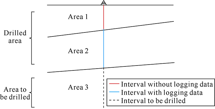
Fig. 2.
Schematic diagram of data structure of well-seismic information integration guided drilling.
In order to improve the accuracy of predicted seismic velocity of undrilled formation, it is necessary to revise and update the seismic velocity of drilled section. The conventional seismic velocity model building method uses grid tomography method to uniformly update the velocity information of the three areas[14]. Adding prior logging velocity information mostly adopts the mode of limiting the update amount of the tomography grid velocity at the well trajectory[15,16,17]. However, this method is more suitable for large-scale 3D seismic velocity modeling, with low computational efficiency and low inversion accuracy for local targets. To solve this, a new velocity updating technology combining the well logging and seismic information has been put forward, in which the updating calculation is simple and efficient.
2.1. Seismic velocity updating of drilled formation
2.1.1. Correction and updating of shallow formation seismic velocity
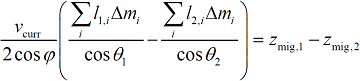
Logging would generally not run in shallow formations. With no logging data available, the seismic velocity of shallow formation is modified and updated by combining the mud-logging horizon and seismic interpretation data. Provided that there are n seismic interpretation horizons in the shallow area, which are marked top-down as 1, 2, ..., n. The one dimension seismic velocity can be updated from top to bottom successively. Assuming that there is a constant multiple error in the velocity of a horizon and the reflection time position by seismic interpretation is equal to the travel time of reflection wave of the real horizon, the velocity updating equation of horizon M in area 1 is as follows:
The updating process of velocity is a recursive process, that is, starting from the surface, the parameters in subsequent layers are calculated recursively. The one-dimensional velocity in the updated shallow area can be obtained following those steps. The updated velocity can make the seismic imaging depth approach to the real depth of the horizon, thus providing a more reliable base for the velocity updating of area 2 and 3.
2.1.2. Reconstruction of seismic velocity in logged sections
The acoustic log data is higher in resolution than seismic data, but different in scale from seismic data. In order to apply it to seismic data processing, it is necessary to reconstruct the low-frequency components of acoustic logging data. Firstly, the median filtering with boundary preserving feature is used to eliminate the abnormal values in acoustic logging data and reduce the scale of acoustic logging velocity to some extent. Then, Gaussian smoothing method is used to adjust the scale of logging velocity through scale factor to make it consistent with seismic scale. Hence, the reconstruction and update of seismic velocity of the logged section can be done.
2.1.3. Geologically constrained interpolation technology
The one-dimensional seismic velocities obtained from the methods mentioned above are spliced and integrated. The overlapping area of two velocities is subject to the one-dimensional seismic velocity model of logged interval. The curve formed by splicing is the updated one-dimensional seismic velocity model of drilled area, which can be extended to three-dimensional space thereafter. Three dimensional velocity modeling of drilled section is a spatial interpolation issue. Many interpolation algorithms can be directly used in the modeling. However, the results obtained from different interpolation algorithms have large differences. After repeated tests, the elliptic equation interpolation algorithm of partial differential equation has the highest accuracy[18]. The specific work flow of modeling under constraint of geologic structure is as follows: (1) Extract geological structure characteristics from the migration profile, and use tensors to express geological structures to facilitate the interpolation process; (2) Use the elliptic equation of partial differential equation to realize structure constrained interpolation; (3) Smooth the interpolation result with structural constraint to remove the false image that may be introduced in the interpolation.
2.1.4. Multi-velocity information integration technology
After the updated seismic velocity model of the drilled area is obtained, it is necessary to integrate this model with the original base seismic velocity model to form a final seismic velocity model of the drilled area. The original velocity model established by the routine method has a relative low resolution. When it is combined with updated seismic velocity model obtained by interpolation, the resolution and accuracy of the seismic velocity model can be improved with the help of high- resolution logging information. Because of large scale and wide range, the original velocity model has an acceptable accuracy in a large scope. While the velocity obtained by logging is of high accuracy only in vicinity of the measured wellbore. With the increase of distance from the well, its accuracy decreases rapidly. The principle of integration is that the closer to the well trajectory, the greater the weight of the interpolation updated seismic velocity model in the integration process is.
The integration method is as follows: firstly, Gabor transformation is used to transform the seismic velocity reference model and the seismic velocity interpolation model into the wave number domain, respectively, and then the two are integrated in the wave number domain. Secondly, the Gabor inverse transformation is used to transform the model back to the spatial domain to get a more accurate velocity model of the drilled area.
Because logging is usually measured in a certain depth interval, the reliability of velocity is not high enough in the interval without logging and in areas with scarce wells. The conventional Fourier transformation is a global transformation, which cannot deal with segment integration. Gabor transformation is a multi-scale time-frequency analysis technology, which can obtain the time-frequency spectrum from time signal. The corresponding integration process in the time-frequency domain can integrate and match the velocity models more accurately, and thus a seismic velocity model with higher accuracy can be obtained.
2.2. Prediction of seismic velocity of the formation to be drilled
In order to improve the efficiency of seismic velocity modeling, the fast tomography method while drilling with simplified parameters is used for the formation ahead of bit. Similar to the principle of conventional tomography method, this method also uses the residual curvature of imaging gathers to update the velocity parameters. But the tomography efficiency is improved the tomography efficiency from the following two aspects: (1) The velocity information of drilled well section has been obtained from the method mentioned above (area 1 and 2 in Fig. 2). Here, only the seismic velocity parameters of the formation to be drilled need to be updated, the conventional tomography technology can be used to update those velocity parameters of the whole area, and the tomography while drilling technology is only used for the velocity parameters in the area to be drilled (Fig. 3). By using the above method, the number of model parameters can be greatly reduced and the efficiency can be improved. (2) The layered description of velocity before drilling can be consistent with the seismic interpreted horizon; if some horizons from seismic interpretation are too thick, they will be divided into multiple horizons.
Fig. 3.
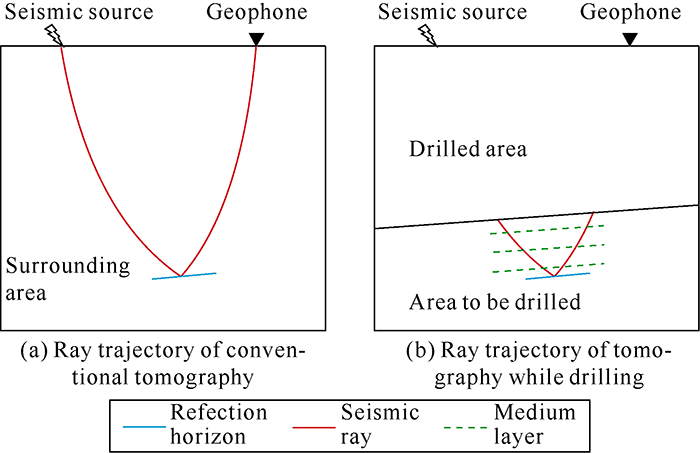
Fig. 3.
Schematics showing differences between conventional tomography and tomography while drilling.
The theory of this method is illustrated using one layer to be updated. The relationship between slow disturbance and depth error in tomography velocity inversion of common imaging point gathers in depth domain[19] is as follows:
Equation (2) needs the true depth parameter of the interface, which cannot be obtained directly. In order to eliminate this limitation, the relationship between the slow disturbance of seismic ray from another reflection angle and the depth error can be established as follows:
In the updated area, the assumed tomography equation of layered medium is established by the difference between equation (2) and equation (3) as below:
where
Equation (4) is a linear equation constructed by single offset information on the imaging gathers. A linear equation group, i.e. tomography equation set, can be constructed using the information of different offsets (i.e. imaging data with different reflection angles) on the imaging gathers. The model parameters c0 and c1 of each horizon can be obtained by solving the tomography equation set. The velocity can then be updated using the following equation:
2.3. Prediction of geological features and description of drilling geological environment factors of the formation to be drilled
The geological features include formation attitude, structure, lithology, fluid etc., and mostly concerned by drilling workers among those features are horizon, lithology, formation dip angle, fault zone, unconformity surface, fracture-cavity formation, etc. Using the updated seismic data, the dip and azimuth attributes can be extracted[20], and used as the constraint condition to extract coherence attributes[21-22] of the seismic data volume to predict the dip angle, positions of faults and fracture zones of the formation to be drilled accurately. The conventional seismic interpretation methods can be used to predict and correct the horizon and lithology of the formation to be drilled to reduce related errors.
Drilling geological environment factors refer to the geological factors that have direct impacts on safe and efficient drilling. These factors mainly include rock drillability, formation pressure (pore pressure, fracturing pressure, and borehole collapse pressure), rock mechanical parameters, potential formation risk factors and basic data in drilling model, etc. By using the corrected high-precision seismic velocity model of the formation to be drilled that further updated by seismic inversion and description method of drilling environmental geological factors[23,24,25,26,27,28,29], these factors of the formation to be drilled can be rapidly described.
Based on the newly predicted geological features, drilling geological factors and possible risks of the formation ahead of the bit, drilling engineers can optimize drilling decisions in advance to avoid or reduce complex down-hole problems which could improve drilling efficiency and reduce drilling cost effectively.
3. Field application
This technique has been applied in seven wells in the Tarim Basin, Songliao Basin and Sichuan Basin since 2019. The whole process of seismic velocity model updating, seismic data reprocessing, geological feature predicting of formation to be drilled and drilling geological environment factor description were all controlled within 20 hours. The technique has worked well in guiding drilling in real time.
Well A in the Longfengshan gas field of the Songliao Basin is a three-stage directional well with a designed drilling depth of 4920 m, a second-section depth of 500 m, a third-section depth of 2969 m, and a kick off point depth of 3350 m in the third section. During drilling, mud loss occurred at 2500 m and 2770 m in the second section, respectively, with a cumulative mud loss of 139 m3, but there was no early warning prompt of leakage in the drilling design. As a large number of cases of lost circulation and wellbore instability were encountered in this area, mud loss and instability risks in the third section were prompted in the drilling design. In order to improve drilling efficiency and ensure drilling safety, well-seismic information integration guided drilling technique was adopted in the third section drilling.
3.1. Correction of velocity model of formation to be drilled and prediction of key geologic horizons
The logging interval of Well A is relatively complete, so only acoustic logging data (without logging horizon information) of the second section was used to reconstruct the 1-D seismic velocity constraint information as shown in Fig. 4. According to the technique of seismic velocity fast updating while drilling, based on the velocity shown in Fig. 4b, a new velocity model of drilled formation (above the second section) was obtained by using the structure constrained interpolation and integrating with original velocity (weight 10.0%).
Fig. 4.
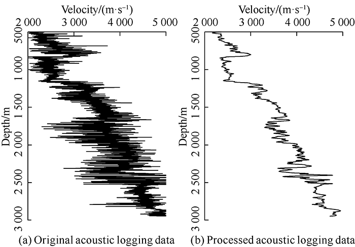
Fig. 4.
Reconstruction of acoustic logging data.
Based on the new velocity model, a velocity model of formation ahead of bit was obtained by using the seismic velocity prediction technology for the formation to be drilled (Figs. 5 and 6). After depth migration, a new seismic profile was formed as shown in Fig. 7. Compared with the original profile, the new seismic profile of drilled formation shows a clearer fault plane at 2480-2600 m, which corresponds well with the actual drilling mud loss point; meanwhile, it can be seen that the formation has obvious lateral changes, the locations of some faults change significantly, and the depths of key horizons also change somewhat accordingly.
Fig. 5.
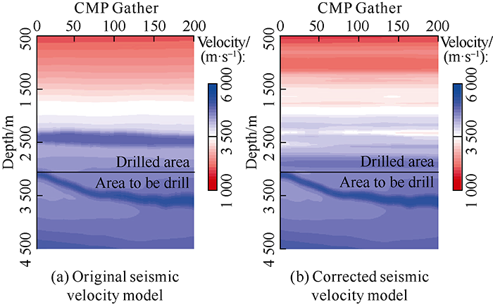
Fig. 5.
Seismic imaging velocity model before and after correction.
Fig. 6.
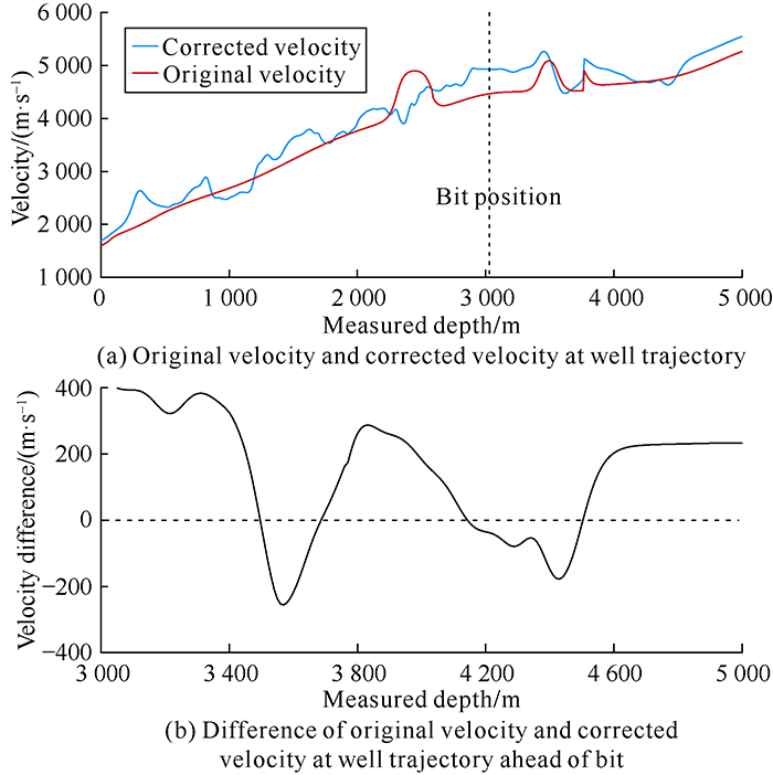
Fig. 6.
1-D seismic velocity model and velocity difference before and after correction along drilling trajectory.
Fig. 7.

Fig. 7.
Seismic imaging profiles before and after correction.
The drilling data of the well shows that the error between the marker horizon interpreted by the original profile and the actual drilling horizon is 91 m, while the marker horizon interpreted from the newly corrected profile is more consistent with the actual drilling depth (Fig. 7), with a much smaller error (23 m). Moreover, the fidelity of new profile is signifi-cantly improved. The coherence attribute profile (Fig. 8) extracted from the new seismic profile indicates that there is no obvious fracture zone in the formation to be drilled. During the third section drilling, there was no fractured leakage, proving that the new engineering geological understanding of no obvious fracture zone has high reliability.
Fig. 8.
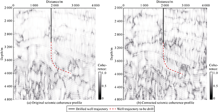
Fig. 8.
Seismic coherence profiles before and after correction.
3.2. Prediction of formation pressure system while drilling and optimization of drilling fluid density
In the drilling design of Well A, the equivalent density of pore pressure in the third section was anticipated at 0.95-1.10 g/cm3, and the designed drilling fluid density was 1.15-1.24 g/cm3. According to the effective stress law and wellbore stability mechanics, the pore pressure, collapse pressure and fracturing pressure of the third section were corrected (Fig. 9). It can be seen from Fig. 9 that this well section was predicted to have a pore pressure coefficient of 1.02-1.12, breakdown pressure coefficient of 1.65-1.83, a wide collapse pressure range, a collapse pressure coefficient of sloughing mudstone section (measured depth of 3720-3950 m and 4310-4600 m) of 1.18-1.38, and an estimated mud loss equivalent density of not less than 1.41 g/cm3. At the same time, in light of the understanding that there is no obvious fracture zone, it was speculated that the potential risk of serious mud loss was relatively small. After comprehensively considering the risk factors such as ROP improvement, hole collapse control and lost circulation, it was decided to increase the drilling fluid density in the third section drilling to 1.24-1.34 g/cm3. In the drilling, polyamine drilling fluid system with strong inhibition was used, there was no mud loss or wellbore issues (in line with the judgment and prediction), and the well was completed after smooth drilling of the third section.
Fig. 9.
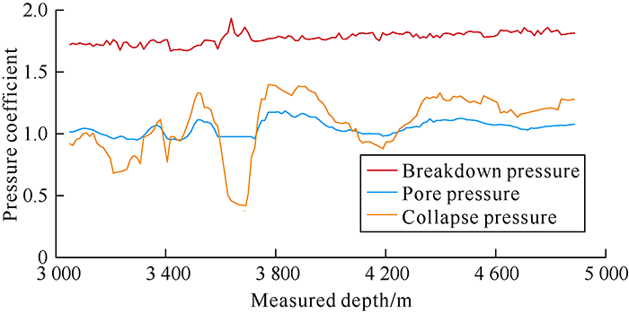
Fig. 9.
Corrected pressure system of the formation to be drilled.
After drilling, the fracturing pressure coefficient measured at 3430 m is 1.67, and the pore pressure coefficient measured at 4850 m is 1.13, proving the predicted accuracy over 90.0%. The average hole enlargement ratio of the mudstone section in this well is 8.70%, which is 12.24% lower than that of the adjacent well (20.94%).
3.3. Drillability prediction while drilling and optimization of bit parameters
According to the updated seismic velocity model, the rock drillability level-value profile of the formation to be drilled in the third section was plotted (Fig. 10). Combined with the imaging results and actual drilling data of adjacent wells, it was predicted that the stratum of basalt and andesite above 3790 m was 5.3-8.7 in drillability; the stratum of interbedded glutenite and mudstone below 3790 m was 5.2-7.2 in drillability. According to the drillability, KPM1642ART and M1655FGA bits were selected, and the optimized drilling parameters were the WOB of 80-100 kN, rotary speed of 50 r/min, flow rate of 28-30 L/s and pumping pressure of 17.5 MPa. The actual drilling has proved that the bits used and optimized parameters worked well in enhancing ROP, with the average ROP in the third section reaching 4.96 m/h, 21.3% higher than that of adjacent wells (4.09 m/h).
Fig. 10.
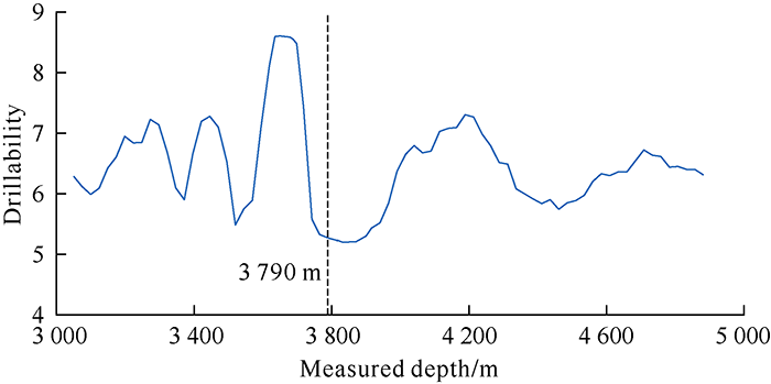
Fig. 10.
Predicted drillability level-value profile of the formation to be drilled in the third section.
The practice of Well A shows that the well-seismic information integration guided drilling plays an important role in optimizing drilling in real time, hence it will have great potential and broad application prospects.
4. Conclusions
The well-seismic integration guided drilling technology mainly include 3 key parts, the update of seismic velocity of drilled formation, prediction of seismic velocity of the formation to be drilled, and the prediction of geological characteristics and description of geological environmental factors of the formation to be drilled.
For the shallow formation without logging data, seismic velocity can be corrected and updated by combining mud logging horizons with seismic interpretation data, so that the seismic imaging depth can be close to the true depth of horizon; for the deep formation with logging data, the low-frequency component of acoustic logging data needs to be reconstructed, and the logging velocity scale can be adjusted consistent with the seismic scale by using Gaussian smoothing method.
In the three-dimensional velocity modeling of drilled section, the elliptic equation interpolation algorithm in partial differential equation can result in quite high precision; after obtaining the seismic velocity model updated by the interpolation of drilled section, the final seismic velocity model of drilled section can be obtained from integration by using Gabor transform and inverse transformation.
The residual curvature of imaging gathers is used to update the velocity parameters of the formation to be drilled, and the fast tomography method with simplified parameters can enhance the efficiency of seismic velocity modeling.
The prediction accuracy of geological features and drilling geological environmental factors ahead of bit can be improved using the corrected seismic image and seismic velocity model.
Field applications show that well-seismic integration guided drilling can predict geological features, drilling geological environmental factors and complex drilling problems ahead of bit timely and reduce the data processing cycle, with much higher efficiency and prediction accuracy. Its prediction results can provide scientific basis for optimizing drilling decision.
Nomenclature
cM―the velocity update coefficient of the M-th layer, dimensionless;
c0―the background parameter of tomography inversion with single layer, s/m;
c1―the perturbation parameter of single layer tomography inversion, dimensionless;
i―stratum number;
l1,i, l2,i―length of reflected rays corresponding to reflection angles θ1 and θ2 in the i-th horizon, m;
m―formation slowness, s/m;
M―seismic velocity updated layer number;
n―seismic interpreting horizon number in shallow area;
Tseis,M―time of seismic interpreting horizon M, s;
vcurr,M―average wellbore trajectory velocity of the M-th layer before updating, m/s;
vupd,i―average wellbore trajectory velocity of the i-th layer after updating, m/s;
z―formation depth, m;
ztrue―actual depth of the formation, m;
zmig,1, zmig,2―the imaging depths corresponding to the reflection angles θ1 and θ2, m;
αi, αM―stratum dips of the i-th and M-th layer, (°);
Δm―formation slowness disturbance, s/m;
θ1, θ2―reflection angle, (°);
φ―stratum dip at reflection point, (°).
Reference
Geology-engineering integration: A necessary way to realize profitable exploration and development of complex reservoirs
Method of calculating drilling parameters
Study on drilling geological environmental factors in Saya Uplifts
Study of formation pressure prediction with seismic interval velocity
Analyzing the formation environmental factors by use of seismic while drilling
Description technology of drilling geological environmental factors and its application
Past, present and future of seismic migration imaging
DOI:10.13810/j.cnki.issn.1000-7210.2015.05.027
URL
[Cited within: 1]

In this paper, we first give a brief review of the history of seismic imaging. Then we discuss the common used migration approaches such as acoustic migrations on P-wave velocity, elastic migrations on both P- and S-wave velocity, anisotropic migrations on three weak anisotropy parameters, and visco-elastic migration on viscosity parameters. Meanwhile, we look at velocity model building and computer hardware developments which are very important for seismic migration. After that, we state some applications of seismic migration imaging in the aspects of structural interpretation, parameter inversion, amplitude attribute extraction, joint analysis of well logging and seismic attributes, and even seismic acquisition design. Finally we anticipate more magnificent achievements of seismic imaging based on elastic, complex anisotropy and visco-elastic prestack depth migrations in the near future era of cloud computing and massive data.
A new fully integrated method for seismic geohazard prediction ahead of the bit while drilling
DOI:10.1190/tle32101222.1 URL [Cited within: 1]
Seismic guided drilling: Near real time 3D updating of subsurface images and pore pressure model
Seismic guided drilling technique based on seismic while drilling (SWD): A case study of fracture-cave reservoirs of Halahatang block, Tarim Oilfield, NW China
An efficient method for drilling trajectory optimization based on seismological and geological guidance of VSP data during drilling and its application
A decade of tomography
High-precision tomography velocity inversion based on well data constraint
DOI:10.11720/wtyht.2015.4.24
URL
[Cited within: 1]
Logging data is considered to be prior information which is fairly accurate and reliable.The utilization of the logging velocity information in the tomographic inverse function system can enhance the precision and efficiency;Nevertheless,it fails to describe the small-scale targets exactly.In view of such a situation,the authors propose a high-precision tomography velocity inversion method based on the well data constraint in this paper.First,the traditional well data constraint tomography velocity inversion is performed.Under the presumption that he velocity of grids in the well position remains the same,the inversion function is establishd based on the well data constraint,the velocity field is updated,and the primary migration image is updated.Second,the logging velocity is used to restrain the migration depth,process velocity analysis and perform precise modeling,thus improving the modeling accuracy greatly.At the same time,the number of the inversion iteration is reduced and the precision is improved.Examples from the synthetic dataset and field data processing demonstrate the feasibility and validity of this method compared with traditional tomography velocity inversion and waveform inversion.
The high-precision tomography velocity inversion method with well control
Tomographic determination of velocity profile and depth in laterally varying media
DOI:10.1190/1.1441970 URL [Cited within: 1]
Image-guided blended neighbor interpolation of scattered data: Image-guided blended neighbor interpolation of scattered data
Common imaging gathers tomography velocity inversion and model building in foothill area
Robust estimator of 3D reflector dip and azimuth
Image structure analysis for seismic interpretation
Eigenstructure-based coherence computation as an aid to 3-D structural and stratigraphic mapping
DOI:10.1190/1.1444651 URL [Cited within: 1]
Methods of obtaining basic drilling parameters using well log information
Methods of selecting drilling bits using well log information
Achieving rock drillability with multi-logging parameters
A method for formation pressure prediction using seismic and logging data
Nonlinear mapping between the characteristic parameters of borehole-side seismic trace and acoustic interval transit times is made by using neural network,then acoustic logging curve under borehole bottom may be obtained through extrapolation to predict formation pressure under borehole bottom by using seismic and loggrog data. This method removes some limitations in formation pressure prediction using only seismic interval velocity or acoustic interval transit times. The modeling prediction of real data in NH area proves that the method brings good effect.
Advances in calculating methods for rock mechanics parameters
Prediction method of regional in-situ stress of oilfield and borehole stability
