

Introduction
With the increasing demand for oil and gas resources, oil and gas exploration and development has gradually expanded to deep layers, deep water/ultra-deep water, and unconventional shale oil and gas resources. Consequently, the drilling conditions have gradually become complex due to downhole high temperature and high pressure, variable reservoir types, narrow pressure windows, and complex well types [1-2]. Under the influence of multiple factors, it is very difficult to control wellbore pressure during drilling and completion, and the risk of leakage and kick accidents is very high. It is very difficult to design the key parameters of well killing. An accurate calculation of wellbore pressure under complex operating conditions requires more accurate wellbore pressure calculations. Gaining deep insights into the law of multiphase flow in the wellbore and developing a highly adaptive wellbore transient multiphase flow model are of great significance to the analysis of the blowout process, formulation of a well-killing scheme, and fine control of wellbore pressure [3].
Numerous theoretical models have been proposed for multiphase flow simulations in wellbores in China and abroad. The drift-flow model is widely used because of its simple and clear mathematical form and good calculation effect [4-5]. The concise governing equation is sensitive to the constitutive equation of the relative motion between the phases, and its solution requires good continuity and mathematical stability. The prediction accuracy of the wellbore drift flow model primarily depends on the closed relationship (in this study, the closed relationship refers to the closed relationship of the drift flow). At present, the closed relationship of the drift flow model is divided into three types: a closed relationship developed based on flow pattern characteristics, a closed relationship of diverging drift flow by introduction of a smoothing function or weighting function, and a single drift flow closed relationship in the full flow pattern domain.
For a closed relationship developed based on flow pattern characteristics, the drift velocity and distribution coefficient of the gas are determined by the drift flow relationship of each flow pattern [6⇓-8]. This type of model has high prediction accuracy for different flow patterns. However, the discontinuity at the transformation boundary of the flow pattern might lead to difficulty in the convergence of the multiphase flow algorithm in transient simulation. The continuity of the closed relationship is solved using the smoothing function or weighting function. However, the resolution of the calculation parameters at the transformation boundary of the flow pattern is low, and the numerical calculation accuracy is decreased. Moreover, different pipe sizes, fluid types, and pipe inclinations have a significant impact on the characteristics of the flow pattern. It is difficult to describe the flow characteristics of variable flow conditions by relying on the characteristics of the flow pattern. The closed relationship of the shunt drift flow has been gradually changed into a single drift flow relationship in the entire flow domain to improve the stability of the numerical calculation of the drift flow model. The closed relationship of the entire flow pattern domain has been changed from the early analysis of the combination of flow pattern characteristics into the way of "theoretical analysis + numerical fitting" [9⇓⇓⇓-13]. The multiphase flow information contained in the closed relationship of the drift flow has gradually increased, ensuring that the multiphase flow in the model is more realistic. Most of these models were developed based on limited experimental conditions or experimental data [12], which is highly dependent on experimental data.
Under the general trend of complex well structures and diversified well killing schemes, the drift flow closed relationship covering the flow characteristics of the full flow pattern domain and with high mathematical continuity has become the key factor for the fine control of wellbore pressure [14-15]. Aiming at the stability and adaptability of the drift flow model, in this study, a multiphase flow experimental database is constructed. In addition, by conducting theoretical analysis and data- driven, a distribution coefficient and gas drift velocity model has been built, which has strong adaptability when the pipe inclination is -90°-90°. The model has been comprehensively evaluated based on the database and well killing cases. The research results can provide theoretical support for the fine control of wellbore pressure and adjustment of the production scheme under complex operating conditions.
1. Drift flow closed relationship
1.1. Multiphase flow experiment database
A database including 3561 sets of gas-liquid two-phase flow experimental data from 32 different data sources, has been constructed. Specific information on the database is shown in Table 1 . The experimental fluid types in this database primarily include air-water, air-kerosene, air-oil, and nitrogen-povidone solutions. The experimental liquid phase viscosity is 0.001-6.880 Pa•s, and the variation range is large in the fluid viscosity during drilling, killing, and production processes. The experimental data containing fluids from low-viscosity to high-viscosity are of great significance in revealing the field flow law. The inclination angle of the experimental pipeline is -90°-90°, covering the flow types from gas-liquid flow in the same direction to gas-liquid flow in the opposite direction. The hydraulic diameter of the pipeline is 0.012 7-0.152 4 m, covering a wide range of flow spaces. The experimental flow pattern includes bubble flow, slug flow, agitation flow, and annular mist flow with gas-liquid flow in the same direction and opposite direction, covering all flow patterns during the production process of oil and gas wells, drilling blowouts, and well killing processes.
| Data sources | Number of data sets | Experimental fluid | Pipe Hydraulic diameter/m | Pipe inclination angle/(°) | Fluid viscosity/ (Pa·s) | Gas content |
|---|---|---|---|---|---|---|
| [14, 16, 19, 21-22, 24-28, 32, 34, 38, 40, 42, 44-46] | 1 794 | Air - water | 0.012 7-0.152 4 | -90-90 | 0.001 | 0.020 0-0.099 8 |
| [17] | 30 | Air - high viscosity oil | 0.050 8 | 0 | 0.187-0.587 | 0.102-0.660 |
| [18, 21] | 250 | Air - mineral oil | 0.050 8 | 28-90 | 0.185-0.213 | 0.149-0.777 |
| [23-24, 33, 35-36, 41, 43] | 954 | Air - kerosene | 0.030 4-0.051 0 | -90-90 | 0.001 3-0.002 0 | 0.006-0.991 |
| [37, 39, 47] | 227 | Air - oil | 0.038 1-0.050 8 | 0-90 | 0.123-0.568 | 0.08-0.89 |
| [26] | 54 | N2 - Luviskol | 0.054 5 | 90 | 0.980-6.880 | 0.08-0.69 |
| [21] | 24 | Air - paraffinic oil | 0.019 0 | 28-90 | 0.035 2 | 0.150-0.589 |
| [19] | 47 | Air - CMC | 0.076 0 | 90 | 0.010 | 0.688-0.963 |
| [20, 29-31] | 181 | Air - Silicone oil | 0.067 0 | 0-90 | 0.005 25 | 0.037-0.894 |
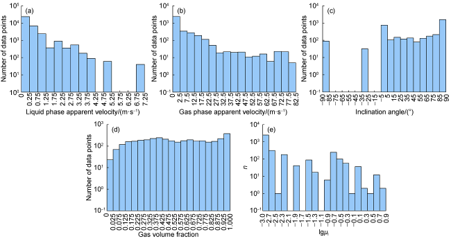
Fig. 1. Data distribution in the built database. |
1.2. Key parameters for drift flow closed relationship
The original concept of the drift flow model was proposed by Zuber et al. [48], which was used to describe the relative slip of gas flow and gas-liquid mixed flow, and revealed the slip difference between the gas and liquid phases in two-phase flow and the gas-liquid two-phase flow in the pipeline distribution law. The gas content and gas drift velocity in the drift-flow model are given by Eqs. (1) and (2), respectively:
$\left\langle {{E}_{\text{g}}} \right\rangle =\frac{\left\langle {{v}_{\text{sg}}} \right\rangle }{{{C}_{0}}\left\langle {{v}_{\text{m}}} \right\rangle +\left\langle \left\langle {{v}_{\text{gm}}} \right\rangle \right\rangle }$
$\left\langle \left\langle {{v}_{\text{gm}}} \right\rangle \right\rangle =\frac{\left\langle {{E}_{\text{g}}}\left\langle {{v}_{\text{g}}}-{{v}_{\text{m}}} \right\rangle \right\rangle }{\left\langle {{E}_{\text{g}}} \right\rangle }$
In the drift flow model, the relationship between the distribution coefficient C0 and gas drift velocity vgm is used to calculate the basic parameter Eg of the two-phase flow in the pipeline. Because these two parameters are unknown, they must be described mathematically, and their key influential parameters must be determined before developing the model of the distribution coefficient and gas drift velocity.
${{C}_{0}}=f\left( \frac{{{\rho }_{\text{g}}}}{{{\rho }_{\text{l}}}},\frac{{{\rho }_{\text{l}}}{{v}_{\text{m}}}{{D}_{\text{h}}}}{{{\mu }_{\text{l}}}},\theta,{{E}_{\text{g}}} \right)$
${{v}_{\text{gm}}}=f\left( {{D}_{\text{h}}},{{\rho }_{\text{l}}},{{\rho }_{\text{g}}},{{\mu }_{\text{l}}},\sigma,\theta,{{E}_{\text{g}}} \right)$
Table 2. Correlation model of drift current relationship |
| References | Distribution coefficient | Gas drift velocity |
|---|---|---|
| [48] | ${{C}_{0}}=1.2$ | ${{v}_{\text{gm}}}=1.53{{\left( g\sigma \Delta \rho /\rho _{\text{l}}^{\text{2}} \right)}^{0.25}}$ |
| [7] | ${{C}_{0}}=1.15$ | ${{v}_{\text{gm}}}=1.53{{\left( g\sigma \Delta \rho /\rho _{\text{l}}^{\text{2}} \right)}^{0.25}}\sqrt{1-{{E}_{\text{g}}}}\sin \theta $ |
| [8] | Bubbly flow: ${{C}_{0}}=1.2-0.2\sqrt{{{{\rho }_{\text{g}}}}/{{{\rho }_{\text{l}}}}\;}\left[ 1-\exp \left( -18{{E}_{\text{g}}} \right) \right]\ \ $ Slug flow: ${{C}_{0}}=1.2-0.2\sqrt{{{{\rho }_{\text{g}}}}/{{{\rho }_{\text{l}}}}\;}\ $ Annular flow: ${{C}_{0}}=1+{\left( 1-{{E}_{\text{g}}} \right)}/{\left( {{E}_{\text{g}}}+4\sqrt{{{{\rho }_{\text{g}}}}/{{{\rho }_{\text{l}}}}\;} \right)\ \ }\;$ | Bubbly flow: ${{v}_{\text{gm}}}=1.41{{\left( g\sigma \Delta \rho /\rho _{\text{l}}^{\text{2}} \right)}^{0.25}}{{\left( 1-E_{\text{g}}^{{}} \right)}^{1.75}}$ Slug flow: ${{v}_{\text{gm}}}=0.35\sqrt{g{{D}_{\text{h}}}\Delta \rho /\rho _{\text{l}}^{{}}}$ Annular flow: ${{v}_{\text{gm}}}=\frac{1-E_{\text{g}}^{{}}}{E_{\text{g}}^{{}}+4\sqrt{{{{\rho }_{\text{g}}}}/{{{\rho }_{\text{l}}}}\;}}\left( {{v}_{\text{m}}}+\frac{\sqrt{g{{D}_{\text{h}}}\Delta \rho \left( 1-E_{\text{g}}^{{}} \right)}}{\sqrt{0.015{{\rho }_{\text{g}}}}} \right)$ |
| [9] | ${{C}_{0}}=\frac{A}{1+\left( A-1 \right)\min \left[ {{\left( \frac{\max \left( {{E}_{\text{g}}},\frac{{{E}_{\text{g}}}\left| {{v}_{\text{m}}} \right|}{{{v}_{\text{sgf}}}} \right)-B}{1-B} \right)}^{2}},1 \right]}$ | ${{v}_{\text{gm}}}=\frac{\left( 1-{{E}_{\text{g}}}{{C}_{0}} \right){{C}_{0}}K\left( {{E}_{\text{g}}} \right){{v}_{\text{c}}}}{{{E}_{\text{g}}}{{C}_{0}}\sqrt{{{{\rho }_{\text{g}}}}/{{{\rho }_{\text{l}}}}\;}+1-{{E}_{\text{g}}}{{C}_{0}}}$ $K\left( {{E}_{\text{g}}} \right)=\left\{ \begin{align} & 1.53/{{C}_{0}}\text{ }{{E}_{\text{g}}}\le 0.2 \\ & {{K}_{u}}\text{ }{{E}_{\text{g}}}\ge 0.4 \\ \end{align} \right.$ ${{v}_{c}}={{\left( g\sigma \Delta \rho /\rho _{\text{l}}^{\text{2}} \right)}^{0.25}}$ |
| [10] | ${{C}_{0}}=\frac{2}{1+{{\left( {R{{e}_{\text{m}}}}/{1000}\; \right)}^{2}}}+\frac{1.2-0.2\sqrt{{{{\rho }_{\text{g}}}}/{{{\rho }_{\text{l}}}}\;}\left( 1-\exp \left( -18{{E}_{\text{g}}} \right) \right)}{1+{{\left( {1000}/{R{{e}_{\text{m}}}}\; \right)}^{2}}}$ | ${{v}_{\text{gm}}}=0.024\,6\cos \theta +1.606{{v}_{\text{c}}}\sin \theta $ ${{v}_{\text{c}}}={{\left( g\sigma \Delta \rho /\rho _{\text{l}}^{\text{2}} \right)}^{0.25}}$ |
| [13] | ${{C}_{0}}=\frac{1.088}{1+0.088\min \left\{ {{{\left[ \max \left( {{E}_{\text{g}}},\frac{{{E}_{\text{g}}}\left| {{v}_{\text{m}}} \right|}{{{v}_{\text{sgf}}}} \right)-0.833 \right]}^{2}}}/{{{1.67}^{2}}}\;,1 \right\}}$ | ${{v}_{\text{gm}}}=\left\{ 1.017{{v}_{\text{v}}}\sin \theta +\left[ 1-\frac{2}{1+{{\text{e}}^{50\sin \left( \theta +2.303{{v}_{\text{m}}} \right)}}} \right]{{v}_{\text{h}}}\cos \theta \right\}\left( 1+\frac{1000}{R{{e}_{\text{m}}}+1000} \right)$ ${{v}_{\text{v}}}=\frac{\left( 1-{{E}_{\text{g}}}{{C}_{0}} \right){{C}_{0}}K\left( {{E}_{\text{g}}} \right){{v}_{c}}}{{{E}_{\text{g}}}{{C}_{0}}\sqrt{{{{\rho }_{\text{g}}}}/{{{\rho }_{\text{l}}}}\;}+1-{{E}_{\text{g}}}{{C}_{0}}}$ ${{v}_{\text{h}}}={{E}_{\text{g}}}\left( 1-{{E}_{\text{g}}} \right)\sqrt{g{{D}_{\text{h}}}}\left( 1.981-1.759\frac{{{N}_{\mu }}^{0.477}}{{{N}_{\text{Eö}}}^{0.574}} \right)$ |
| [12] | ${{C}_{0}}=\frac{2-1.07E_{\text{g}}^{\text{1}\text{.3}}}{1+{{\left( {R{{e}_{\text{m}}}}/{1\text{ }000}\; \right)}^{2}}}+\frac{1.2-0.205E_{\text{g}}^{\text{5}\text{.8}}}{1+{{\left( {1\text{ }000}/{R{{e}_{\text{m}}}}\; \right)}^{2}}}$ | ${{v}_{\text{gm}}}=\left( 0.45\cos \theta +0.35\sin \theta \right)\sqrt{g{{D}_{\text{h}}}}{{\left( 1-{{E}_{\text{g}}} \right)}^{0.75}}$ |
1.3. Drift flow closed relationship construction
1.3.1. Gas drift velocity model
1.3.1.1. Influence of pipe inclination
The gas drift velocities at pipeline inclination angles of 0 °to 90° are mostly constructed based on the gas drift velocities in the horizontal and vertical pipelines. The gas drift velocities at the two extreme angles are both proportional to $\sqrt{g{{D}_{h}}}$. The proportionality coefficient is determined based on experimental and theoretical studies. Potential flow theory yields proportional coefficients of 0.35 and 0.45 for vertical and horizontal conditions, respectively [11,49]. In this study, when constructing the gas drift velocity model, considering the influence of the pipe inclination angle and pipe diameter on the gas drift velocity, the two basic terms Aθ and ADh of the model are constructed.
${{A}_{\theta }}=0.35\sin \theta +0.45\cos \theta $
${{A}_{{{D}_{\text{h}}}}}=\sqrt{\frac{g{{D}_{\text{h}}}\left( {{\rho }_{\text{l}}}-{{\rho }_{\text{g}}} \right)}{{{\rho }_{\text{l}}}}}$
Aθ in Eq. (5) is established for a pipeline inclination angle of 0° to 90°, which cannot solve the two-phase flow problem in the full inclination angle range. When the pipeline is turned from the horizontal to the inclined downward position and the gas flow rate is low, the tail of the gas phase becomes sharp owing to the buoyancy effect and tends to move in the opposite direction of the two-phase flow. Bendiksen [50] found that when the inclination angle is -30°≤θ<0°, the gas drift velocity has a negative value (i.e., the direction of the two-phase flow is opposite) when the velocity of the gas-liquid mixed fluid is less than the critical velocity. When the gas phase Froude number Fr is less than 0.1, the gas phase migration velocity is lower than the critical velocity. When the gas phase velocity exceeds the critical velocity, the gas content in the pipeline is high, and the gas phase drift velocity is not affected by the direction of the pipeline. Based on the above analysis, Bhagwat et al.[11] proposed a sign reversal criterion: while satisfying the inclination angles of -50°≤θ<0° and Fr≤0.1, the sign of the gas drift velocity was reversed from positive to negative. However, this model is not continuous, which increases the convergence difficulty of the numerical algorithms. Here, the Fourier transform is used to construct a sign-reversed continuous function that simultaneously satisfies the dip angle range of -50°≤θ<0° and Fr≤0.1; the dip angle sign switching function (Eq. (7)) and Froude number switching function (Eq. (8)) are combined to establish a continuous functional relationship that simultaneously satisfies the above two conditions.
${{C}_{\theta }}=1-\frac{2{{C}_{Fr}}}{1+{{e}^{50\sin \left( \theta +0.08 \right)}}}+\frac{2{{C}_{Fr}}}{1+{{e}^{50\sin \left( \theta +0.872 \right)}}}$
${{C}_{Fr}}=\left\{ \begin{align} & \frac{1}{1+{{e}^{50\sin \text{ }\left( {Fr}/{0.1}\;-1 \right)}}}\text{ }Fr<0.4 \\ & 0\text{ }Fr\ge 0.4 \\ \end{align} \right.$
1.3.1.2. Effect of liquid viscosity
The liquid viscosity has a significant effect on the flow pattern distribution, and the viscous force also has a strong effect on gas slippage [51-52]. Experimental results have revealed that liquid viscosity has a considerable effect on the gas drift velocity under different pipeline inclination angles. [49]. It can be observed from Table 2 that most models ignore the influence of liquid viscosity, and the prediction adaptability is significantly reduced. Therefore, when predicting the gas drift velocity, liquid viscosity must be introduced into the model. Schlumberger used the viscosity number to calculate the effect of fluid viscosity on gas drift velocity [13]. Based on this idea, this study optimizes the gas drift velocity by making the viscosity dimensionless (μl/μw) and introduces a new viscosity term, Cμl:
${{C}_{{{\mu }_{\text{l}}}}}=1-0.036\ln \left( \frac{{{\mu }_{\text{l}}}}{{{\mu }_{\text{w}}}} \right)$
1.3.1.3. Influence of interference between gas groups
In a gas-liquid two-phase flow, there is mutual interference between bubble groups, which is different from the gas drift velocity of a single bubble. Shoham [53] introduced liquid holdup El to revise gas drift velocity. The correction form of El0.75 is widely used in gas drift velocity prediction models[11⇓-13]. Based on the analysis of the experimental data, this study adopts the modified gas drift velocity with El0.5 to consider the influence of interference between bubble groups, and the sum of the liquid content and gas content is one.
1.3.1.4. Influence of pipe diameter and surface tension
The gas drift velocity is positively correlated with the pipe diameter. However, it is unreasonable that the gas drift velocity is infinite when the pipe diameter is infinite. As the pipe diameter increases, the gas tends to diffuse laterally, and the lateral expansion of the gas increases the upward resistance and reduces the magnitude of the increase in the gas drift velocity. The induced resistance of the pipe wall is negatively correlated with the diameter of the pipe. With the increase in the diameter of the pipe, the influence of the induced resistance of the pipe wall on the gas-phase motion gradually weakens. When a certain critical size is exceeded, the influence of pipe diameter on the gas drift velocity can be ignored. The upper limit of the rising velocity of the gas is affected by the critical pipe size and interfacial tension. In the latest research by Schlumberger, the Eotvos number NEö was used to limit the increase in gas drift velocity [13]. In this study, referring to Schlumberger's ideas, NEö is used to construct the limiting term of the gas drift velocity, and the influence coefficient CNEö of the Eotvos number is obtained by fitting the experimental data.
${{C}_{{{N}_{\text{Eö}}}}}=\left\{ \begin{align} & {{\left( \frac{\sqrt{{1}/{{{N}_{\text{Eö}}}}\;}}{0.025} \right)}^{0.15}}\text{ }{{N}_{\text{Eö}}}>1\text{ }600 \\ & 1 \ \ \ \ \ \ \ \ \ \ \ \ \ \ \ \ \ \ \ \ \ \ \ \ \ \text{ }{{N}_{\text{Eö}}}\le 1\text{ }600 \\ \end{align} \right.$
Based on the above analysis, a gas drift velocity relationship is proposed considering the pipe inclination, pipe diameter, fluid physical parameters, and gas content.
${{v}_{\text{gm}}}={{A}_{\theta }}{{A}_{{{D}_{\text{h}}}}}{{C}_{\theta }}{{C}_{{{N}_{\text{Eö}}}}}{{C}_{{{\mu }_{\text{l}}}}}{{\left( 1-{{E}_{\text{g}}} \right)}^{0.5}}$
1.3.2. Distribution coefficient model
Before determining the relationship between the distribution coefficient and flow parameters in Eq. (3), it is necessary to perform quantitative and qualitative analysis about the influence of different factors based on experimental data in the database. Data statistical analysis involved the experimental data of many researchers. Owing to the advancement of multiphase flow monitoring technology, there are significant differences in experimental conditions, and the accuracy of the experimental data will be different. In addition, there will be certain deviations in the experimental data under similar parameter conditions. When using an experimental database for quantitative analysis, the data must first be screened for validity.
The previous model is used to screen valid data. First, the model of Liu et al. [12] is used to compute the gas drift velocity and distribution coefficient under all the experimental conditions, and data with a distribution coefficient of less than 1 are screened out. Subsequently, the selected data are calculated using the models proposed by Choi et al. [10] and Shi et al. [9] to calculate the gas drift velocity and distribution coefficient. Data with a distribution coefficient of less than 1 are screened out. After completing the above operation, the data points that deviated significantly from the whole are deleted under the same experimental conditions. The data analysis and model development in this study are based on the screened 3016 sets of experimental data.
1.3.2.1. Influence of viscosity
By comparing the prediction results of the theoretical model in Table 2 with the data in the database, it is found that the distribution coefficient predicted by the model is 1.0 to 1.2, which only satisfies the distribution coefficient range when the bubble flow changes into the annular mist flow under the low-viscosity condition and underestimated the high-viscosity condition. The range of distribution coefficients is below 1.0 to 2.0. To improve the applicability of the distribution coefficient relationship in a larger viscosity range (low viscosity-high viscosity), it is necessary to further investigate the influence of viscosity on the distribution coefficient. The intuitive influence of viscosity is reflected by the Reynolds number (Rem=ρlvmDh/μl). The variation law of the distribution coefficient with Reynolds number is illustrated in Fig. 2 a. As the fluid viscosity increases, the fluid disturbance decreases. Due to the side lift force, the bubbles tend to move towards the center of the pipe. In addition, the bubble at the center of the pipe has the highest rising speed. The distribution coefficient can be used to characterize the uneven distribution and velocity of bubbles in the pipe section. The higher the degree of bubble aggregation in the center of the pipe, the greater the distribution coefficient. The distribution coefficient is higher (over 2.0) under the condition of a low Reynolds number, which is lower than the conventional value (1.2 in viscous fluids). Under the condition of a high Reynolds number, the fluid turbulence effect is strong, and the bubble movement is affected by the turbulent vortex. In summary, the influence of the fluid viscosity on the distribution coefficient is primarily reflected in the turbulence degree in the gas-liquid two-phase flow. The Reynolds number is used to explain the variation in the distribution coefficient as follows[12], where the first term represents the low Reynolds number term and the second term represents a high Reynolds number term:
${{C}_{0}}=\frac{A}{1+{{\left( {R{{e}_{\text{m}}}}/{1\,\,000}\; \right)}^{2}}}+\frac{B}{1+{{\left( {1\,\,000}/{R{{e}_{\text{m}}}}\; \right)}^{2}}}$
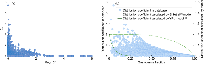
Fig. 2. Correlation analysis of distribution coefficient. |
1.3.2.2. Influence of pipe inclination
The inclination angle of the pipeline affects the gravity system of the two-phase fluid, and the gas distribution in the pipeline changes with the inclination angle. When the fluid in the pipeline gradually changes from vertical upward flow to horizontal flow, the distribution coefficient exhibits a decreasing trend. When the flow direction continues to change downward, the gas has two migration directions, and the gas distribution also changes with the migration direction and change. Therefore, B0 is used to characterize the effect of the inclination, as shown in Eq. (13).
${{B}_{0}}=1.2{{\left\{ {\left[ 1+{{\left( {{{\rho }_{\text{g}}}}/{{{\rho }_{\text{l}}}}\; \right)}^{2}}\cos \theta \right]}/{\left( 1+\cos \theta \right)}\; \right\}}^{0.2\left( 1-{{E}_{\text{g}}} \right)}}$
1.3.2.3. Influence of gas content
The gas phase distribution in the two-phase flow is closely related to the flow pattern in the pipeline, and the gas content is the most critical parameter for characterizing the flow pattern, and it is strongly related to the distribution coefficient. Fig. 2 b depicts the correlation between the distribution coefficient and gas content in the database, and the variation trend of the distribution coefficient with gas content predicted using the Shi et al.[9] and YPL (Yield-Power-Law) models [12]. The correlation between the distribution coefficient and gas content predicted by Shi et al. [9] exhibits a convex function, which is inconsistent with the change law of the experimental data. Although the YPL model underestimated the distribution coefficient, it could reflect the change in the distribution coefficient with gas content. This variation trend was better than that of the model of Shi et al. Therefore, the YPL form in Eq. (14) can describe the evolution law of the distribution coefficient in the entire flow pattern relatively accurately.
${{C}_{0}}={{X}_{1}}+{{X}_{2}}{{E}_{\text{g}}}^{{{X}_{3}}}$
Considering these factors comprehensively, the distribution coefficient equation under the influence of fluid viscosity is composed of a low Reynolds number term and a high Reynolds number term. The term replaces the X1 term in YPL form, constructing a new distribution coefficient equation:
${{C}_{0}}=\frac{A-{{\left( {{{\rho }_{\text{g}}}}/{{{\rho }_{\text{l}}}}\; \right)}^{2}}}{1+{{\left( {R{{e}_{\text{m}}}}/{1\text{ }000}\; \right)}^{2}}}+\frac{{{B}_{0}}+{{X}_{2}}{{E}_{\text{g}}}^{{{X}_{3}}}}{1+{{\left( {1\text{ }000}/{R{{e}_{\text{m}}}}\; \right)}^{2}}}$
Using data from the multiphase flow experiment database, Eq. (15) is parametrically analyzed. With the goal to minimize the average error between the calculated gas content and the actual gas content, optimization is done. Finally, the constant coefficients A, X1, and X3 are obtained as 2.0, -0.2, and 6.8, respectively.
1.3.3. Model performance
In Eq. (15), the influence of gas content, pipe inclination, and fluid physical parameters has been considered comprehensively, covering a wide range of multiphase flow conditions. In this study, in the drift flow model, multi-parameters and multi-source data have been integrated. It is necessary to analyze the model stability to ensure that the model has good continuity, with stable and reasonable predicted values on physical parameters.
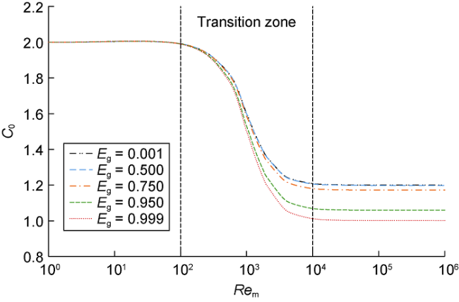
Fig. 3. Influence of gas content on distribution coefficient. |
With the increase in well depth, the physical parameters of the gas phase change. The increase in gas density has a significant influence on the distribution law of the gas-liquid two-phase. Fig. 4 illustrates the variation in the distribution coefficient with the Reynolds number for different gas-liquid density ratios. In contrast to the gas content, the influence of gas density on the distribution coefficient is primarily concentrated in the low-Reynolds- number range. As the density ratio increases, the slippage effect of the gas phase weakens, and the distribution of the gas-liquid two-phase tends to be uniform; thus, the distribution coefficient decreases. When overflow occurs in deep and ultra-deep wells, the gas drift velocity and distribution coefficient change during the gas rising process. It is difficult to accurately predict the change in wellbore pressure using conventional distribution coefficient models.
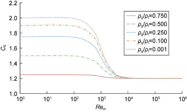
Fig. 4. Influence of density ratio on distribution coefficient. |
The inclination angle of the pipeline affects the gas drift velocity and distribution, which subsequently affects the gas content. The control of wellbore pressure in the inclined well and extended-reach horizontal well is depended on the sensitivity and stability of the model. Fig. 5 a depicts the predicted gas content at different inclination angles. The pipe diameter was set to 0.05 m, the liquid viscosity was 0.001 Pa•s, and the liquid superficial velocity was 0.5 m/s. With an increase in the absolute value of the inclination angle, the gas content decreased, primarily because of the enhanced slippage effect of the gas under the action of gravity. The gas changed from a uniform distribution to a concentrated distribution in the center of the pipeline, which increased the distribution coefficient and decreased the gas content [11]. Simultaneously, the rheology of the fluid in the wellbore affects the drift law of the gas and the boundary of the flow pattern transformation. To control precisely the wellbore pressure, it is required that the model should have a high sensitivity to fluid viscosity. Fig. 5 b presents the predicted gas content of fluids with different viscosities in the vertical pipeline as a function of the gas superficial velocity. The pipe diameter was 0.05 m and liquid superficial velocity was 0.5 m/s. When the fluid viscosity increased, the Reynolds number of the gas-liquid miscible fluid decreased significantly, the distribution coefficient increased, and the gas content decreased.
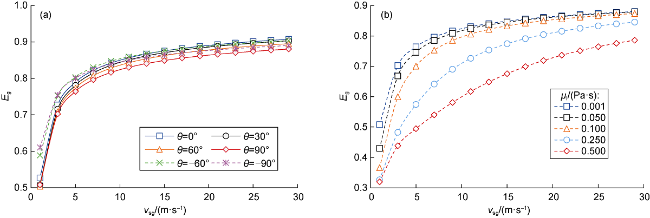
Fig. 5. Influence of pipeline inclination and fluid viscosity on predicted gas content. |
2. Model validation and application
2.1. Drift flow model verification
Using the multiphase flow experimental database established in this study, the drift-flow relationship proposed in this study and the drift-flow relationship proposed by Liu et al. [12], Choi et al. [10], and Hibiki et al. [8] are predicted and evaluated. The model prediction results are shown in Fig. 6 and Table 3 . The prediction results under the fog flow are the best for different models, and the data points are concentrated within the error range of ±20%. The prediction results with the model in this study and those of Hibiki et al are within the error range of ±10%. The reason for the poor prediction results with the model of Choi et al. [10] is that the predicted value of the distribution coefficient is too high under the condition of annular flow, affecting the calculation of gas content. All the models have abnormal discrete points for the prediction of bubbly and slug flows. With the same structural form, the prediction results on bubbly and slug flows have high points with the models in this study, the model by Liu et al. [12], and the model by Choi et al. [10]. The primary reason is that when the Reynolds number is low, the estimated value on the distribution coefficient is low, whereas the drift flow relationship of Hibiki et al. [8] is established based on the flow pattern, which has different deviations for different flow pattern degrees. To quantitatively analyze the prediction results of the drift- flow relationship, the average residual ε1, average relative error ε2 and standard deviation ε3 are used to statistically analyze the model calculation results.
${{\varepsilon }_{1}}=\frac{1}{N}\sum\limits_{i=1}^{N}{\left| {{E}_{\text{g,pred}}}-{{E}_{\text{g,meas}}} \right|}$
${{\varepsilon }_{2}}=\frac{1}{N}\sum\limits_{i=1}^{N}{\left| \frac{{{E}_{\text{g,pred}}}-{{E}_{\text{g,meas}}}}{{{E}_{\text{g,meas}}}} \right|}$
${{\varepsilon }_{3}}=\sqrt{\frac{1}{N}\sum\limits_{i=1}^{N}{\left| \left( {{E}_{\text{g,pred}}}-{{E}_{\text{g,meas}}} \right)-{{\varepsilon }_{1}} \right|}}$
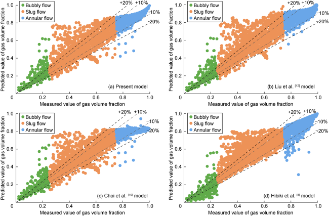
Fig. 6. Comparison between predicted and measured values of gas content with different models. |
Table 3. Prediction results of different drift current relationships |
| Models | Proportion of data points within ± 20% error range | Proportion of data points within ± 10% error range | ε1 | ε2 | ε3 |
|---|---|---|---|---|---|
| Present model | 80.86% | 62.63% | 0.057 8 | 0.132 9 | 0.065 2 |
| Liu et al. model[12] | 76.36% | 57.49% | 0.069 1 | 0.154 5 | 0.083 3 |
| Choi et al. model[10] | 80.00% | 43.56% | 0.081 7 | 0.164 0 | 0.076 1 |
| Hibiki et al. model[8] | 75.56% | 57.92% | 0.066 2 | 0.155 7 | 0.083 9 |
2.2. Application of drift flow relationship in wellbore multiphase flow
2.2.1. Transient drift flow model solution
Another factor affecting the prediction accuracy of the wellbore drift flow model is the numerical solution format of the nonlinear system of equations. The finite volume method deals with multiphase flow equations by means of integration, and is superior to the finite difference method in terms of physical conservation, computational stability, and robustness, and has been widely used in computational fluid dynamics and fluid engineering in recent years. In this study, the finite volume method of a staggered grid is used to deal with the space convection term of the multiphase flow equation system. The convection term of the first-order upwind style discrete multiphase flow governing equation is selected, and the unsteady term of the first-order backward difference scheme discrete governing equation is selected. Referring to the processing method of interface parameters by Wang et al. [14], a pressure prediction-correction solution framework for a multiphase flow equation is developed based on the semi-implicit method for the pressure-linked equation (SIMPLE)-like method coupled with the field algorithm of wellbore temperature proposed by Liao et al.[15], to realize unsteady multiphase flow simulation in wellbore.
2.2.2. Bullheading killing simulation
The drift flow model established in this study covers the flow situation with an inclination angle of -90° to 90° and has certain guiding significance for well killing simulation under different working conditions. To verify the adaptability of the wellbore drift flow model established in this study, simulation was conducted for a well in the Tarim Oilfield with bullheading killing method (pipeline inclination of -90° to 80°). The relevant parameters for this well are listed in Table 4 .
Table 4. Relevant parameters of a well in Tarim |
| Parameter | Value | Parameter | Value |
|---|---|---|---|
| Casing inner diameter | 200.0 mm | Drilling fluid density | 1.2 g/cm3 |
| Casing running depth | 6 384 m | Drilling fluid viscosity | 30 mPa·s |
| Drill pipe od above 2480 m | 114.3 mm | Kill fluid density | 1.94 g/cm3 |
| Outer diameter of drill pipe deeper than 2480 m | 88.9 mm | Kill fluid viscosity | 25 mPa·s |
| overflow quantity | 6.4 m3 | Well depth | 7 241.4 m |
The reservoir section of this well is a carbonate fracture-cave type reservoir controlled by faults. During the drilling process, sudden overflow occurred. When the well was shut in, the drilling fluid pool increased by 6.4 m3, and the wellhead pressure was 41.8 MPa after the well was shut in. Affected by the gas composition, a good killing strategy of annular hydraulic injection was adopted. The displacement was first pressed back to a displacement of 20 L/s to ensure the safety of the wellhead, and then the displacement was increased to 24 L/s. The entire killing process was simulated using the model in this study, and the simulation results are illustrated in Fig. 7 . The wellhead casing pressure was 42.88 MPa when the well was shut for 24 min. At this time, high-density killing fluid (1.94 g/cm3) was injected from the annulus at a displacement of 20 L/s, and the wellhead casing pressure increased rapidly to 54.24 MPa. After entering, the back pressure of the wellhead gradually decreased. At 40 min, the killing displacement increased to 24 L/s, and the wellhead casing pressure suddenly increased to 47.30 MPa. With the displacement of the killing fluid and pressure of the gas back into the formation, the wellhead casing pressure gradually decreased. After the killing fluid reached the bottom of the well, the pressure-back method was completed, and the back pressure at the wellhead was stabilized at 2.61 MPa. The figure clearly shows that the calculation results of the model are highly consistent with the field data. The calculation error of the casing pressure at shut-in was 2.58%, the calculation error of the casing pressure at the initial pressure was 3.43%, and the calculation error of the casing pressure when adjusting the displacement was 5.35%.
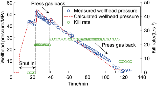
Fig. 7. Wellhead pressure change during well killing by back pressure method. |
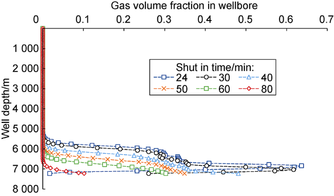
Fig. 8. Variation of wellbore gas content at different times during backpressure. |
3. Conclusions
In wellbore multiphase flow, the gas drift velocity is primarily affected by the pipe dip angle, pipe diameter, fluid physical property parameters, and gas content. The distribution coefficient is primarily affected by fluid viscosity, pipe dip angle, and gas content. Based on theoretical analysis, with data-driven approach, we have established the gas-liquid two-phase drift flow relationship model with a full flow pattern and full dip angle, which has good continuity. With this model, we can obtain stable and reasonable prediction values of the physical parameters. Moreover, through comparison the calculation results of the model with the database data, it has been found that with the model established in this study, the proportions of predicted data volume within the ±20% and ±10% error limits are 80.86% and 62.63%, respectively, and the standard deviation of the prediction error is 0.065 2. Compared with the existing model, the model established in this study has the highest prediction accuracy and prediction stability. For the flow conditions with the pipeline dip angle of -90° to 80°, the simulation error of the casing pressure at shut-in is 2.58%, the simulation error of the initial pressure back casing pressure is 3.43%, and the prediction error of the casing pressure when the displacement is adjusted is 5.35%. The calculation results of the model under the flow conditions are in good agreement with the field.
By using drift-flow relationship in this study, we have solved the problem that the split-flow model is difficult to converge and has low computational efficiency when simulating unsteady multiphase flow. It has high stability under complex flow conditions. It is of great significance in guiding the fine control over wellbore pressure, and safe production operations.
Nomenclature
Aθ—influence coefficient of pipe inclination, dimensionless;
ADh—influence coefficient of pipe diameter, m/s;
A, B—constant coefficient in the relationship between Reynolds number and distribution coefficient, dimensionless;
B0—influence coefficient of pipe inclination, dimensionless;
CFr—influence coefficient of Froude number, dimensionless;
${{C}_{{{N}_{\text{Eö}}}}}$—influence coefficient of Eotvos number, dimensionless;
Cθ—influence coefficient of pipe inclination, dimen-sionless;
${{C}_{{{\mu }_{\text{l}}}}}$—influence coefficient of fluid viscosity, dimen-sionless;
C0—distribution coefficient, dimensionless;
Dh—hydraulic diameter, m;
Eg—gas volume fraction, dimensionless;
Eg,pred—predicted gas volume fraction, dimensionless;
Eg,meas—measured gas volume fraction, dimensionless;
El—liquid content, dimensionless;
f—function;
Fr—froude number, dimensionless;
g—gravitational acceleration, m/s2;
i—serial number of experimental data;
K—correlation coefficient of gas drift velocity, dimensionless;
Ku—kutateladze number, dimensionless;
n—number of data points;
N—total experimental data;
NEö—eotvos number, dimensionless;
Nμ—viscosity number, dimensionless;
Rem—reynolds number of gas-liquid mixture, dimensionless;
vc—single bubble migration velocity, m/s;
vg—the true velocity of the gas, m/s;
vgm—gas drift velocity, m/s;
vh—gas migration velocity in horizontal pipe, m/s;
vm—gas-liquid mixed fluid speed, m/s;
vsg—gas phase apparent velocity, m/s;
vsgf—flooding velocity, m/s;
vv—gas migration velocity in vertical pipeline, m/s;
X1, X2, X3—constant coefficient in YPL model, dimensionless;
Δρ—gas liquid density difference, kg/m3;
ρg—gas phase density, kg/m3;
ρl—liquid density, kg/m3;
μl—viscosity of liquid phase, mPa•s;
μw—viscosity of water, mPa•s;
σ—surface tension, N/m;
θ—inclination of pipe, rad;
ε1—average residual;
ε2—average relative error;
ε3—standard deviation;
$\langle \rangle $—section average flow characteristics;
$\langle \langle \ \rangle \rangle $—section weighted average flow characteristics.