

Introduction
During the long-term development of oil fields, the pressure-temperature conditions of oil occurrence and its composition changes significantly. As a result, the dissolving ability of oil in relation to asphaltenes may decrease, which leads to their flocculation. The flocculation of asphaltenes in oil generally does not lead to severe consequences under the production. Nevertheless, precipitated asphaltenes then turn into solid deposits, which have a high adsorption capacity. Therefore, during filtration, they are deposited onto the surface of the porous medium of the rock, reducing the hydraulic radius of pore channels, and creating filtration resistance, which leads to formation damage[1]. The complication of modeling these mechanisms is that the reservoir has a complex structure of the porous medium.
Simulating the before-mentioned processes has become possible by activating the asphaltene option in the compositional dynamic simulator. The simulator allows us to consider the loss of thermodynamic equilibrium in the oil when modeling different reservoir production modes under dynamic conditions with uncertainties. The simulator further acts as a tool for reservoir engineers to make important management decisions when monitoring field development. Knowledge of the phase transition conditions of asphaltenes in oil allows a reasonable approach to choosing a reservoir production scheme along with well operation conditions to minimize production risks. A number of researchers have used compositional simulators to simulate asphaltene deposition, proposed a number of models to describe asphaltene behavior, and studied the mechanisms of formation damage caused by asphaltene deposition [2-3].
Compositional dynamic simulation using the asphaltene option is a relatively new topic that has begun to gain more and more popularity in recent years due to the fact that new models for describing the asphaltenes behavior in oil are emerging and the mechanisms of the formation damage are constantly being developed.
The novelty of this paper lies in the fact that for the first time sensitivity analysis and uncertainty evaluation were performed when modeling the asphaltenes deposition in the porous medium of one of the Russian oil field using a compositional reservoir simulator and own data from special laboratory studies of oil and core samples. Until now, different authors only using the reservoir properties have carried out the uncertainty evaluation. In this paper, the authors used the parameters of the asphaltene option to analyze the uncertainties in order to assess how the combined effect of all parameters of the asphaltene option and their ranges influence the oil production in the field.
1. Reservoir modeling
The history of the development of the oil field considered in this paper is almost 46 years long. The first stage of the field development was accompanied by intensive drilling. As a result, 240 wells were drilled in the field (216 are production wells and 24 are injection wells). The wells were drilled in the highest oil-saturated thicknesses and were placed in three rows along the main axis of the field on a grid of 400 m × 500 m. The process of creating a field model is described below.
1.1. Static modeling
The authors created a static model of the studied field, its size along the main axis is 19 km and along the secondary axis of 5 km. The construction of the main structural frame of the static model of the field was carried out along the top and bottom of the pay zone in its stratigraphic boundaries. The identification of the stratigraphic boundaries of the reservoir was carried out according to data obtained using following complex of geophysical methods: nuclear logging, self-potential method, and resistivity logging. Well logging diagrams were compared with the data of the adjacent wells. The correlated interlayers were investigated according to the typical configuration of well logging curves, taking into account the sequence of the deposit formation and the features of the facies structure of the studied area. The linear dimensions of the cells of the geological grid were chosen, taking into account the area of the field and the average distance between the wells. In doing so, the condition of placing at least five grid cells between adjacent wells on the area of the production facility in the horizontal plane was fulfilled. Thus, the cell sizes are taken as 50 m × 50 m, and the number of vertical layers and their sizes are selected, considering the minimum thickness of permeable interlayers (0.5 m). The porosity cube was calculated according to the interpretation of the well logging data, presented in the form of the Kp curve (porosity). The spatial distribution of porosity was conducted by interpolation of well data using a 3D model. In order to calculate the oil saturation cube, the Ko curve (oil saturation) was utilized, obtained from logging data, taking into account a specific position of oil-water contact. The reservoir is characterized by average porosity and permeability values: 0.19 and 0.8 μm2, respectively. The average initial oil-saturated thickness is 30 m.
1.2. Dynamic modeling
The oil reservoir was enclosed entirely in a geological grid, together with a part of the aquifer. The simulation of the waterdrive system was carried out by increasing the pore volume of the near-boundary water-saturated part of the reservoir. When building the dynamic model of the field, the Corner Point method was chosen. The grid of the dynamic model was generated using the up-gridding of the static model. The up-gridding model of the field was carried out only vertically. The number of vertical layers and their sizes were determined, considering the compartmentalization of the layers. Interlayers of dense rocks, significant in area, were distinguished during the up-gridding into separate layers. Thus, the dimensions of the cells were 50 m × 50 m × 3.6 m. The full-scale dynamic model consists of more than 1 100 000 cells. The reservoir properties for the enlarged grid of the dynamic model were obtained from the performed upscaling operation. A sector with dimensions of 1.5 km × 1.5 km (from the central part of the reservoir) was cut from the full-scale model to reduce the calculation time. The pattern consists of 33 000 cells. Only four production wells were included in the pattern (Fig. 1 ). The aquifer in the pattern was tuned to restore the dynamics of pressure and production in this section of the reservoir.
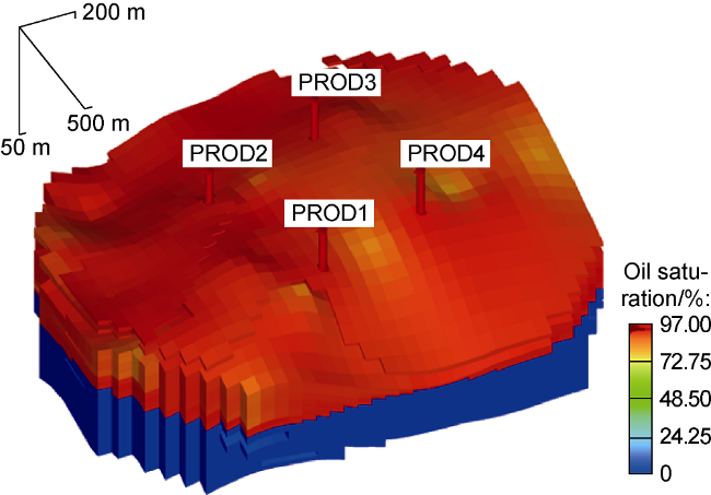
Fig. 1. Pattern of the dynamic model. |
Complex processes, such as water coning, asphaltene deposition, amongst others, require large discretization of the computational grid in limited regions of interest. Using refined grid subdivisions of the entire model may not be achievable due to the time needed for the calculation. In addition, the use of refined grid in areas minimally affected or not affected by these processes is impractical. This problem can be solved by using the local grid refinement method proposed by Heinemann et al.[4]
Refinement starts at the uninvaded area (original grid) and ends with the region of interest. In this case, each subsequent cell adjacent to the previous one is refined no more than two to three times until the required grid size in the region of interest is reached [5]. This rule is used to achieve the required accuracy in calculating the flow between the original and the refined grid blocks.
Local grid refinement was carried out in the area of each production well. At a distance of 75-125 m from the well, the original grid in the horizontal plane was split in half (i.e., the size of the new grid was 25 m×25 m), at a distance of 25-75 m from the well, the original grid was split fourfold (i.e., the size of the new grid was 12.5 m× 12.5 m), and at a distance of 0-25 m from the well, the original grid was split eight times (i.e., the size of the new grid was 6.25 m×6.25 m). In the vertical plane, the original grid was halved in the considered area of interest (i.e., the size of the new grid along the z-axis was 1.8 m). The local grid refinement around the production well is shown in Fig. 2 .
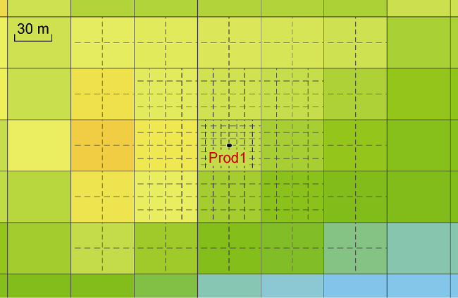
Fig. 2. Local grid refinement around the production well. |
The relative permeabilities used in the dynamic model are shown in Fig. 3 .
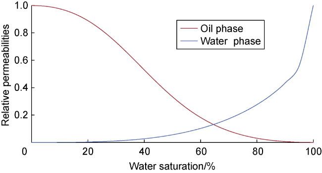
Fig. 3. Relative permeabilities. |
1.3. PVT-modeling
Based on the results of laboratory PVT analyzes, a PVT model of the oil field was built using Soave-Redlich- Kwong EOS. The model used the Lorenz-Bray-Clark viscosity calculation method. Parameters such as critical temperature and pressure, acentric factor, volume shift factor, binary interaction coefficients, and others have been tuned for laboratory studies. The PVT model was tuned for experimental results with an error of less than 1%.
The composition of oil in the model was grouped into seven pseudo-components: N2 and C1 were grouped into a single component X1, since they have similar thermodynamic properties; CO2, C2, and C3 were grouped into component X2 since CO2 shows similar behavior with intermediate light oil components; components C4 through C6 were grouped into a single component X3; components C7 to C14 were grouped into a single component X4; components C15 to C21 were grouped into a single component X5; the rest of the components (C22 +) were grouped into the X6 component. The heaviest oil component, C22+, was split into non-settling component X6nA (high molecular weight paraffinic hydrocarbons) and settling component X6A (asphaltenes). The composition of oil and the properties of the components are presented in Table 1 . The components containing asphaltenes have high binary interaction coefficients compared to the non-settling components (Table 1 ). This explains its lower compatibility with light oil components.
Table 1. Oil composition and component properties |
| Component | Molar fraction | Molecular mass/ (g·mol-1) | Critical temperature/ °C | Critical pressure/ MPa | Acentric factor | Critical volume/ (m3·mol-1) | Parachor | Conversion coefficient of volume | Specific gravity | Binary iteration coefficients |
|---|---|---|---|---|---|---|---|---|---|---|
| X1 (N2+ C1) | 0.088 80 | 22 | -112 | 4 | 0.025 | 0.094 | 59 | 0.137 | 0.555 | 0 |
| X2 (CO2+C2-C3) | 0.166 90 | 39 | 61 | 5 | 0.160 | 0.144 | 112 | -0.626 | 0.560 | 0.981 02 |
| X3 (C4-C6) | 0.204 90 | 72 | 196 | 3 | 0.236 | 0.306 | 228 | 0.585 | 0.626 | -0.258 45 |
| X4 (C7-C14) | 0.235 46 | 145 | 366 | 2 | 0.453 | 0.576 | 419 | 0.575 | 0.758 | 0.821 95 |
| X5 (C15-C21) | 0.120 18 | 252 | 490 | 1 | 0.722 | 1.013 | 691 | -0.589 | 0.818 | -0.841 77 |
| X6nA (C22+) | 0.181 70 | 449 | 665 | 1 | 1.109 | 1.806 | 1229 | 0.640 | 0.875 | 0.336 18 |
| X6A (C22+) | 0.002 06 | 600 | 704 | 1 | 1.009 | 2.469 | 1135 | 0.474 | 0.950 | 0.420 48 |
Results of the laboratory experiments of the constant composition expansion (CCE) are shown in Fig. 4 . 20 MPa is the reservoir pressure, 6.8 MPa is asphaltene onset pressure (AOP), a bubble-point pressure is 4.7 MPa. Oil viscosity in reservoir conditions is 2.6 mPa•s. The oil density at surface conditions is 840 kg/m3.
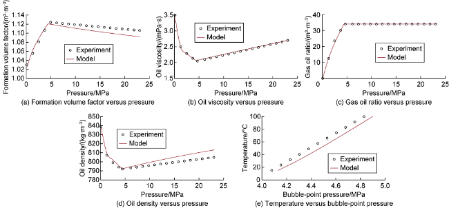
Fig. 4. Results of the laboratory experiments of the constant composition expansion. |
The asphaltene flocculation model in the PVT simulator was tuned according to the results of investigations carried out in the authors previous studies [6]. The aim of the previous investigation was to evaluate the asphaltene onset pressure. The experiment was a decrease in pressure from the reservoir pressure to the asphaltene onset pressure at reservoir temperature. It is known that asphaltenes can also precipitate from oil during temperature reduction at constant pressure. However, the authors did not consider this process since the production of the considered field is carried out without changing the reservoir temperature. The authors were interested in solely those processes that occur under actual reservoir conditions. The rest of the terms are of interest only for academic purposes. In this paper, the authors refer to the source to clearly show the readers that asphaltenes precipitate out at a pressure of 6.8 MPa. However, the current investigation is not laboratory oil studies but is based on them to build correct PVT model and reservoir simulation model. At the AOP, asphaltenes flocculate in the oil, and as the pressure decreases further, they grow in size and settle on solid surfaces, causing difficulties in the oil recovery. As such, it is recommended to maintain reservoir pressure above the AOP.
1.4. The asphaltene option
Ghadimi et al. [7] showed that the activation of the asphaltene option in the compositional dynamic simulator, depending on the production conditions of the field, its size, time of the calculation period, as well as the parameters of flocculation and asphaltene deposition, allow us to take into account a decrease in the oil recovery factor (ORF) by an average of 20%-35%.
The model of asphaltene deposition in the porous medium was tuned to the results of filtration experiments and porous medium studies conducted in the authors previous paper [6] (Figs. 5 and 6 ). The laboratory-adjusted coefficients representing the deposition of asphaltenes in the porous medium were accepted as the base values.
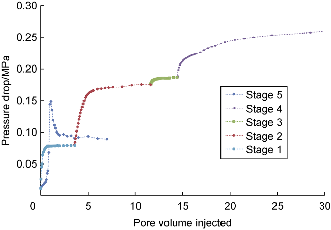
Fig. 5. Pressure drop versus pore volume injected for different back pressures [6]. |
The studies presented in the Figs. 5 and 6 were carried out by the authors in 2019 as part of another scientific research. The purpose of the previous study was to show by filtration and micro computed tomography methods that when asphaltenes are deposited in a porous medium, the diameter of the pore channels decreases. The experiment consisted of two cases: (1) Filtration of oil with dissolved asphaltenes and (2) Filtration of oil with precipitated asphaltenes through a core sample followed by micro computed tomography of the core. Undoubtedly, the accumulated frequency in both cases should be equal to 100%.
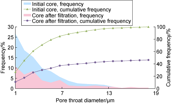
Fig. 6. Pore throat diameter distribution before and after filtration [6]. |
Nevertheless, in the previous paper, the authors wanted to show that, in the case of oil filtration with precipitated asphaltenes, not the absolute accumulated frequency but the relative accumulated frequency is relative to the filtration of oil with dissolved asphaltenes. In this case, the difference in the accumulated frequencies between the two cases shows what percentage of the pore channels is occupied by asphaltene deposits, which more clearly demonstrates formation damage. In this paper, the authors refer to the source to clearly show the readers that asphaltenes are indeed deposited in the porous medium of the rock under the studied conditions, which may occur during field production. However, the present investigation does not consist of laboratory studies of oil filtration and core micro computed tomography but only is based on them to correctly set the asphaltene option in the reservoir simulation model.
In the dynamic simulator, the state of asphaltenes in oil is set in a simplified form. Generally, it is presented in tables containing the dependences of the mole fraction of suspended asphaltenes in oil (percentage of the total asphaltenes amount in oil) on pressure, temperature, and mole fraction of the oil component of interest or the injected chemical. These dependencies are obtained during laboratory studies of oil (asphaltene deposition curve). This approach makes it possible to perform adequate accuracy calculations with a minimum design power and time cost. These tables are created in specialized programs for creating PVT models.
The adsorption, desorption, and plugging coefficients are set by the users based on the results of specific laboratory experiments (dependence of the decrease in core permeability on the number of pore volumes of injected oil with suspended asphaltenes) or history matching of the dynamic model. The mechanism for calculating the deposition of asphaltenes in the porous medium is as follows:
(1) The pressure in each cell is calculated.
(2) The system of conservation equation of the flow is solved, the number of moles of each component in each active cell is determined.
(3) The pressure in the considered area is compared with a given table of the concentration of the suspended asphaltenes versus pressure. Thus, the concentration of the solid phase at the considered cell of the reservoir is determined.
(4) The asphaltene deposition rate over the time intervals is calculated.
(5) Adsorption, desorption, and plugging coefficients are inserted into the asphaltene deposition model, oil saturation at the reservoir point and local porosity are used.
(6) The filtration rate is calculated.
(7) Knowing the asphaltene deposition rate over time, the volume of asphaltene deposition in the porous medium is calculated.
(8) From the initial porosity, the volume of deposits is subtracted, and the local porosity is obtained, from which the permeability is subsequently determined using well- known dependencies. If the filtration rate exceeds the critical rate, then part of the deposits is desorbed from the pore surface and is entrained with the oil flow through the pore channels towards the bottom hole of the producing well.
(9) Oil saturation and pressure are recalculated.
(10) The calculation cycle is repeated.
2. Uncertainty evaluation
The approach to the initial feasibility study of new potential assets in poorly investigated areas (greenfields), especially in the absence of analogous fields, is based on the uncertainty evaluation and has already become standard practice for reservoir engineers [8]. The reservoir in question has a highly complex porous medium structure, which results in static parameters of uncertainty. For the most part, static uncertainties can be referred to as the uncertainties of the reservoir's geological parameters due to the lack of knowledge and the absence of the field development history. They are unchanged throughout the entire history of field production. The above- mentioned analyses make it easy to perform with modern dynamic simulators. At the stages of exploration and preparation of the field for production, it is possible to confirm or disprove the accuracy of the estimations and correct further investment decisions. In the case of potential asphaltene deposition in the field, dynamic uncertainty parameters that change over time are added to the static ones. When capital investments have already been made, the field development strategy has been adopted, the wells have been drilled, and the entire development system has been formed, for various reasons, problems might arise during the field production, which can occur according to various scenarios. Learning about the nature of those issues can be time-consuming due to the demand for expensive special laboratory experiments (along with routine laboratory analysis).
The purpose of the initial assessment of the potential of a poorly studied asset is to estimate the project's risks before starting a full-scale investment. This is no small task for development engineers due to the limited experience working with unknown assets and the unique status-quo of individual reservoir systems and fluids during reservoir development. A satifactory solution to this problem can be achieved by applying multi-variable calculations (MVC). The MVC approach allows us to carry out a comprehensive assessment of investment projects in the conditions of uncertainties in order to make optimal management decisions and minimize financial losses. In the MVC approach, uncertainties are understood as the possibility of any parameter (geological, PVT, filtration, technological, etc.) to take a value that can vary over a wide range due to the measurement error of instruments, methods, research techniques, coverage scale, and other circumstances. Uncertainties of various kinds can have different effects on the final results. In this case, the uncertainty evaluation is the transformation of the uncertainty of the initial data into the uncertainty of the final result. One of the key objectives of the MVC approach is to investigate the field of uncertainties, as well as to evaluate all possible scenarios for hydrocarbon production in the field and the individual and cumulative contribution of uncertainty parameters to production. As we have already mentioned, hydrocarbon production is fraught with all kinds of uncertainties. Starting from the exploration cycle and ending with the field production, several uncertainties are entirely eliminated. In addition, the range of uncertainty parameters is significantly narrowed due ongoing research, obtaining new information about the objective reservoir, and the transition from a macro level of knowledge to a micro-scale of knowledge.
When the field is being drilled out, core sampling and their study, as well as the analysis of formation fluids, geophysical studies and well tests, are carried out. The entire set of studies will form the base of the initial data laid down in the dynamic model. Depending on the equipment, methods, and research techniques, each parameter carries a certain determination error. At the stage of loading data into the model, the error in several parameters can reach 20%, which will unpredictably affect the final results when it comes to the conventional modeling approach. The approach can be simplified as follows: one geological implementation of the model corresponds to one dynamic implementation of the model and one predicted oil production profile.
The initial data are investigated. Based on the error values of the measuring instruments, the accuracy of the research methods, and the scale, covering in this research, the uncertainty parameters are determined, the ranges of their variation and their distribution functions are also estimated. Inaccurate estimation of the ranges of the input parameters with the most influence will lead to incorrect uncertainty evaluation results. The result of the preparation of the initial data for the MVC is a matrix of uncertainty parameters.
Consequently, a sensitivity analysis is carried out, which consists of optimizing the number of input parameters, specifically, determining uncertainty parameters with the most influence on the objective function (the definition will be given in the history matching section), assessing their mutual influence, and excluding from further calculations the remaining non-influencing parameters by carrying out a small number of calculations that are performed using special methods for desinging experiments.
2.1. Experimental design techniques
It is recommended to start a sensitivity analysis with the one variable (OVAT) method [9], which allows us to evaluate the interaction between input and response parameters and identify the parameters with most influence (heavy hitters). If m parameters of uncertainty vary, the number of experiments N is calculated by the formula: N = 2m + 1 (including the base model). Each parameter is sequentially varied (the minimum, base, and maximum values are set in turn), while the rest of the parameters take the base values. Therefore, a response surface is formed, which in this method is a straight line.
After the sensitivity analysis, we move on to the uncertainty evaluation and directly to the multivariate calculations. One of the common methods for designing experiments for performing multivariate calculations is the Latin hypercube, proposed by McKay et al. in 2000 [10]. Using this method, a response surface of a complex shape (usually a polynomial) is obtained, also called a proxy model, describing the entire system's behavior. This method can estimate all parametric space with a fewer number of experiments set by the user. In this case, the possible values of all uncertainty parameters are considered uniformly (the entire range of parameters is used), avoiding the appearance of “empty” areas. For N experiments, the range of each parameter is divided into N levels of equal probability. Then N experiments randomly fill the parametric space with the following restrictions: each experiment occupies a random place on the level, only one experiment occurs at each level. The number of experiments N is in the following range: 5 m < N <20 m. The user can set the number of experiments, but they should be enough to build a complete proxy model.
The algorithm for carrying out multivariate calculations consists of the following stages:
(1) Create a matrix of uncertainty parameters (a set of input parameters with ranges of their variation and distribution probability) and create an objective function (the definition will be given in the history matching section).
(2) Create experiments with low-level designing methods (OVAT, Plackett-Berman), calculate these experiments.
(3) Create a response surface, plot a Pareto chart to determine the most significant input parameters (heavy hitters).
(4) Adjust the ranges of the uncertainty parameters and remove the parameters that do not affect the objective function.
(5) Create experiments using the higher-level designing method (Latin Hypercube) from the input parameters defined in the previous step. Calculate them.
(6) Repeat steps 4-5 until the objective function is minimized.
(7) Create a response surface (proxy model).
(8) Make a blind selection of input parameters, perform calculations on the proxy model with the selected parameters, and check the proxy model's reliability.
(9) Create a set of experiments using the Monte Carlo method. Calculate these experiments using the proxy model built in step 7.
Due to the large amount of information, items 7-9 are not covered in this paper.
2.2 History matching
The dynamic model should become a digital twin of actual field studies and fully reproduce that field’s characteristics (all historical data on well performance) so as to reliably predict future production. This is the aim of the history matching process. History matching is an iterative process of correcting/selecting reservoir parameters (from the approved range obtained during the research) to improve matching operation parameters calculated and historical values. In this case, the criterion for the quality of one dynamic model in comparison with another is the objective function. The history matching process is reduced to minimizing the objective function, which is the difference between the calculated and historical values of the response parameters. The response parameters are, generally, the flow rates of oil, water, gas, cumulative oil, water, gas, and others are set.
Since the studied field belongs to a brownfield with a long production history, over which many core and fluid studies were carried out, the main uncertainties regarding the geological parameters of the reservoir and the properties of fluids can be removed. First, a traditional history matching (static geological parameters of the reservoir) was carried out with a full-scale model without activating the asphaltene option.
During the first stage of history matching, the dynamics of reservoir pressure was recreated, and the fluid production discrepancy value for the field as a whole was minimized. To this end, the following adjustments were made to the input data: (1) correction of pore volumes of water-saturated cells (aquifer); (2) correction of permeability in good areas with large fluid production discrepancy; (3) clarification of wells’ perforation intervals.
The second stage of history matching consists of adjusting the water cut dynamics of the object (the functions of relative permeabilities were adjusted) and obtaining a satisfactory agreement between the calculated technological parameters of the operation of each well and the actual data. The relative permeabilities curves were generated, considering the data of laboratory flooding experiments (determination of the relative permeability and endpoints of the relative permeability depending on the permeability of the core). It also characterizes the dynamics of the water cut of production wells.
During the next stage, the asphaltene option was activated with the base parameters obtained from the results of laboratory tests. Then, from the full-scale model matched at the previous stage, a pattern was cut out, and a historical period was calculated on it. As a result, the boundary conditions were established at the boundaries of adjacent pattern models. We analyzed the model's sensitivity to the parameters of the asphaltene option, based on the results of which we selected the most influencing parameters, to the objective function (the definition is given below).
Consequently, a multivariate history matching was carried out using only the parameters of the asphaltene option to select the correct ranges of variations of the asphaltene parameters. Five hundred calculations were carried out, designed according to the Latin Hypercube method. Based on the results of multivariate history matching (dynamic parameters of the asphaltene option), calculations were selected with an acceptable deviation of the calculated technological parameters from the historical ones (within 10%) - that is 100 calculations. The corresponding range of changes in the asphaltene parameters was split up, and 500 forecasts were generated on their basis (by the Latin Hypercube method) before prediction profile was calculated.
The objective function for multi-variable history matching is:
$F=\sum_{i} \sum_{j=1}^{N_{i}} W_{i} W_{i, j}\left(\frac{Y_{i, j}-Z_{i, j}}{\sigma_{i}}\right)^{2}$
Similar to the methods of designing experiments, the number of response parameters in the objective function should not be too large to optimize the history matching process time. Still, at the same time, it should be sufficient to obtain a good history matching.
After tuning the parameters of the dynamic model of the field according to the development history, it is possible to determine measures designed to optimize and intensify the operation of wells for the forecast period and correct the system for further reservoir development.
As a result of multivariate history matching, a set of tuned (with acceptable accuracy) model variants is obtained, on which forecast calculations are performed. The result is a range of expected production profiles given the input data. Then a probabilistic assessment is made, i.e., determination of percentile probabilities: P10, P50, P90, which show the probability in percentage, with which, it is possible to obtain a certain production profile for the forecast period.
Thus, using the MVC approach allows the company to assess risks when making design decisions under uncertain conditions. It should be noted that the conventional approach (obtaining one forecast production profile) lacks any probabilistic assessments.
3. Results and discussion
3.1. Sensitivity evaluation
The uncertainty parameter matrix in this paper consisted of 11 variables. The range of variation of the asphaltene option parameters was selected based on a literature analysis [7]. For sensitivity analysis, 25 experiments were performed using the Plackett-Burman method to determine the input parameters of most influence on the objective function and assess their mutual impact. The calculation results (for the historical period) of the obtained experiments are shown in Fig. 7 . Variables that correspond to values below 0.05 on the Pareto diagrams do not affect the objective function, so they were excluded from further calculations. Among the selected variables, the most influencing the objective function were A3, A4, A5, G, N, and S, which took part in the MVC.
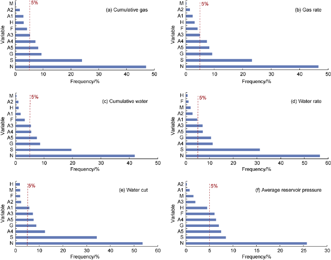
Fig. 7. Pareto diagram of asphaltene parameters in study area. A1, A2, A3, A4, A5—determine the molar weight fraction of dissolved asphaltenes as a function of pressure (with five respective pressure values); S—adsorption coefficient of asphaltenes; F—the desorption coefficient of asphaltenes; G—the critical velocity of oil movement in the reservoir; H—the coefficient of pore-clogging; M—the asphaltene flocculation rate; N—the dissociation rate of asphaltenes. |
3.2. The field production under natural depletion
The Latin hypercube method was used to create 500 experiments from the selected 6 variables at the stage of sensitivity analysis. The calculations were carried out in the natural depletion case. Fig. 8 shows the results of calculations for cases without considering asphaltene deposits and probabilistic profiles (percentiles P10, P50, and P90) with deposits. The oil production rate was used as a control parameter. Over the historical period, the deviation of the cumulative oil production from the actual one was 0. The cumulative gas and water production deviation for the P50 case is less than 5%, for the P10 and P90 cases are less than 10%.
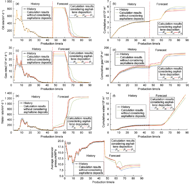
Fig. 8. Calculation results for natural depletion cases. |
The amount of asphaltene deposits precipitated increases in cases P90, P50, P10. The effective pore volume of the reservoir, in this case, decreases with the growth of asphaltene deposition; consequently, the average reservoir pressure also increases in cases corresponding to P90, P50, P10. For the case without deposits, the total fluid production is lower than the one from the P10 case. Therefore, the average reservoir pressure is higher for this calculation as compared to other cases. The uncertainty evaluation results showed that taking into account the asphaltene option provides a reasonable risk assessment of the production parameters for the field. For cases P90, P50, and P10, the cumulative oil production is lower than those from the cases without deposits by 4.0%, 8.1%, and 12.3%, respectively.
At some distance from the production well, where the pressure drops below AOP during production, asphaltenes in oil begin to flocculate. Subsequently, as they reach the well, they adsorb onto the surface of the pore space, as on a filter. The drawdown cone extends from the well into the depth of the reservoir. The driving force of flocculation of asphaltenes in oil increases with a decrease in pressure. Furthermore, the largest pore volumes of fluid with suspended asphaltenes are filtered through the cell, penetrated by the well. Near the well, the asphaltene deposition rate is the highest (Fig. 9 ). However, as oil is filtered from the uninvaded area to the well, the amount of suspended asphaltenes in oil decreases according to the Langmuir adsorption isotherm. Therefore, in the uninvaded area from the well to the constant pressure equal to AOP, the process of asphaltene adsorption also takes place. The deposition of asphaltenes is observed practically throughout the section opened by perforations in the well.
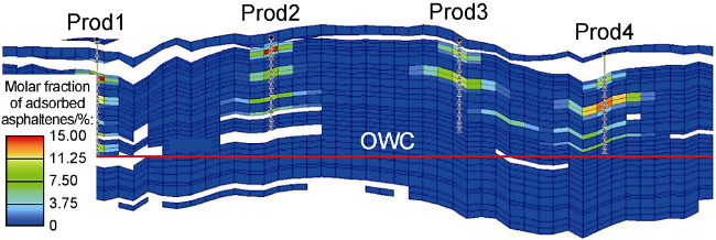
Fig. 9. Map of molar fraction of adsorbed asphaltenes in porous media for natural depletion case at the end of the forecast (Р50). |
3.3. The field production under waterflooding
In order to maintain the energy of the reservoir and prevent asphaltene deposition from spreading deep into the reservoir, it is necessary to organize a waterflooding system that will allow oil to be produced at pressures above the AOP for an extended period. An uncertainty evaluation was carried out to assess the impact of a water flooding system on the results. The analysis was based on 500 experiments created by the Latin Hypercube method from variables (based on the results of sensitivity analysis), having the most influence on the objective function (the same experiments were calculated as in the natural depletion case). The water flooding system in the sector was represented by one injection well drilled in the center of the sector. The well was perforated in the reservoir's aquifer and was brought into production only for the forecast (no injection was performed during the historical period). In this case, the current production compensation by injection was set equal to 1. The calculation results are shown in Fig. 10 .
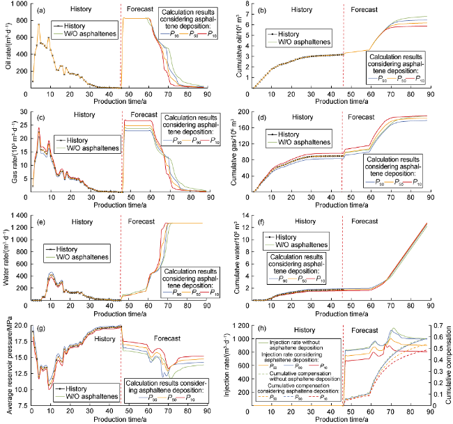
Fig. 10. Calculation results for water flooding cases. |
As in the natural depletion case, with the organization of a water flooding system, the amount of asphaltene deposited increases gradually in cases corresponding to P90, P50, P10, the average reservoir pressure also increases gradually in cases corresponding to P90, P50, P10. For the cases corresponding to P90, P50, and P10, the cumulative oil production is lower than those in the case without deposits by 4.8%, 9.1% and 13.3%, respectively.
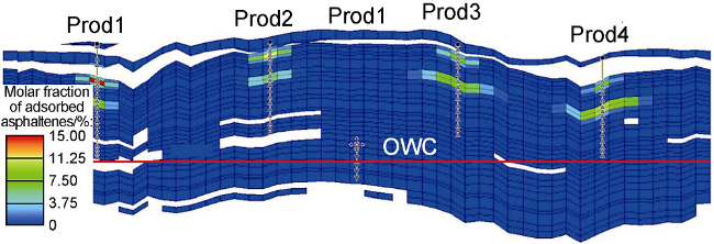
The calculation results showed that the asphaltene deposition in the porous medium significantly reduces the cumulative oil production. In addition, the injection of water (into the reservoir's aquifer) to maintain reservoir pressure can effectively slow down the process of asphaltene flocculation in oil (Figs. 9 and 11 ) and improve the technological efficiency of the field production. Asphaltene deposition is observed in a smaller volume compared to the natural depletion case (Fig. 11 ) and is mostly closer to the top of the reservoir since reservoir pressure is compensated for in the bottom part by water injection. With this conclusion, the authors wanted to say that the water injection into the aquifer of the reservoir allows the reservoir pressure to be maintained above the asphaltene onset pressure for a longer period of time than the operation of the field under natural depletion. This directly affects the amount of deposited asphaltenes in the porous medium of the reservoir. The slower the pressure declines from the initial reservoir pressure towards the asphaltene onset pressure, the slower the formation of asphaltene deposits in the porous medium will be, and ultimately fewer of them will be observed. Thus, in this case, there will be less filtration resistance to the flow of oil from the reservoir into the wells, making it possible to produce more oil. This statement is supported by Figs. 8-11. In this regard, the authors did not mean that water injection directly affects the asphaltenes precipitation through direct interaction with them, leading to physical or chemical processes/reactions. The dynamic simulator assumes that water is chemically inert to asphaltenes.
Fig. 11. Map of molar fraction of adsorbed asphaltenes in porous media for water flooding case at the end of the forecast (Р50). |
Yaseen and Mansoori[11] showed that when oil interacts with emulsified water, the solubility of asphaltenes in oil decreases and asphaltenes begin to flocculate. In this case, strong emulsions may form. The authors considered the case of water injection in oil column. This type of water injection allows performing two main goals: to maintain reservoir pressure at the initial level, and to displace oil in the direction from injection wells to producing ones.
The authors in this paper consider the injection of water in aquifer, just to maintain the reservoir pressure. The oil-water contact rises gradually without the formation of water coning. Thus, the additional interactions of oil with water become smaller compared to the injection of water in oil column. In addition, careful water prepa-ration (mineralization control, addition of surfactants, pre-heating before injection) eliminates undesirable effects with the deposition of asphaltenes (requires additional laboratory investigations for compatibility of the injected water with reservoir oil and rock). Additionally in this paper, the authors made the following assumptions: water does not have any physical or chemical interactions with oil (the formation of emulsions, a decrease in the solubility of asphaltenes in oil, etc.), there is no change in the wettability of the rock due to the deposition of asphaltenes, the oil relative permeability changes only due to changes in the local absolute rock permeability, there is no change in the viscosity of oil from the concentration of suspended solid particles of asphaltenes.
The influence of asphaltenes deposition on the mechanism of oil displacement by water is complex and requires individual investigation. Kamath et al. [12] showed that asphaltene depositions improve the efficiency of oil displacement by water due to the following factors: hydrophobization of the surface of the porous medium due to a layer of asphaltene deposits and an increase in the oil relative permeability. However, at the same time the absolute permeability of the rock decreases.
Attar et al. [13] represented that the water injection in oil column is characterized by less cumulative oil production compared to the water injection in the aquifer, which is associated with more intensive asphaltenes deposition. The authors carried out their calculations on a pattern model cut from a full-scale dynamic model with double porosity.
4. Conclusions
A sensitivity analysis of the pattern model to the input parameters of asphaltene option allowed determining the most influential parameters on the objective function as follows: the molar weight of dissolved asphaltenes as a function of pressure, the asphaltene dissociation rate, the asphaltene adsorption coefficient and the critical velocity of oil movement in the reservoir, above which the dissociation of asphaltenes takes place.
The probable production profiles were evaluated for two cases: with and without the asphaltene option being activated. The calculations were carried out for two production scenarios: the operation of the field under natural depletion and the water injection into the aquifer of the reservoir to maintain the reservoir pressure.
Five hundred uncertainty evaluation cases were calculated with different the asphaltene option parameters in the natural depletion and in the water-flooding scenarios. The results showed that for cases P90, P50, and P10 with deposits, the cumulative oil production in the natural depletion scenario is lower than those in the case without deposits by 4.0%, 8.1%, and 12.3%, respectively. With implementation of the reservoir pressure maintenance system for cases P90, P50, and P10 with deposits, the cumulative oil production is lower than those in the case without deposits by 4.8%, 9.1%, and 13.3%, respectively.
Under depleted production conditions, the reservoir pressure drops significantly and a pressure drop funnel forms, resulting in the deposition of asphaltenes in the bottom hole of the production well and a reduction in productivity. Water flooding can keep the reservoir pressure above the initial precipitation pressure of asphaltenes for a long time and delay the formation of asphaltene deposits in porous media. Compared with oil layer water injection, water layer water injection makes other effects of oil and water (such as the interaction of crude oil and emulsified water reduces the solubility of asphaltenes and accelerates the precipitation of asphaltenes) relatively smaller, which can inhibit the deposition of asphaltenes, so the cumulative oil production is higher.
Acknowledgements
We acknowledge Dr. A.V. Petukhov for his assistance during reservoir modeling. Finally, we would like to thank Saint-Petersburg Mining University for providing computing capacity for performing multi-variable calculations.
Nomenclature
F—objective function for multi-variable history matching;
i—response parameter;
j—the number of the time step at which the value of the corresponding response parameter was observed;
m—number of parameters;
N—number of experiments;
W—weighting factor;
y—the calculated value corresponding to the response parameter i at the time step j;
z—observable value corresponding to the response parameter i at the time step j;
σ—the standard deviation of the response parameter i, determined from the available historical data.