

Introduction
The oil production of an oil well is a critical indicator for oilfield development, and forecasting future production is the key for analysis of reservoir development performance. The variation of single well production is influenced by many factors, such as reservoir properties and stimulation measures. The key to achieving an accurate single well production prediction is to consider each factor fully and carefully, and to grasp the characteristics of the change of production. Compared with the traditional production prediction methods, such as decline curves and numerical reservoir simulation, the machine learning methods have strong nonlinear fitting capability, with high efficiency, and have great application potential in production prediction.
In the past 20 years, a lot of researches have been conducted on the oil production prediction based on machine learning [1⇓-3]. The commonly used algorithms include random forest (RF) [4], support vector machine (SVM) [5-6], fuzzy evaluation (FE)[7], artificial neural network (ANN) [8], etc. With these methods, the oil production is predicted by regressing the relationship between production and its influencing factors, but without consideration of temporal variation in production. Since 2015, recurrent neural network (RNN) represented by long short-term memory (LSTM) and gated recurrent unit (GRU) has become a new hot spot in the field of oil production prediction [9-10]. Compared with classical algorithms such as SVM and RF, RNN focuses on the temporal variation of production. Although the training time has increased significantly, the prediction accuracy has been improved greatly.
For the prediction of single well production with multiple influencing factors, long history span and parallel sequences, previous researchers only used a few features to build prediction models. To further improve the prediction accuracy of single well production, it is necessary to comprehensively consider both dynamic and static influencing factors and build a multi-features production prediction model. When the number of the features is increased, it is hard for RNN to extract high-dimensional spatial information and temporal information at the same time, with limited prediction accuracy. Therefore, it is necessary to use a new algorithm to gain accurate prediction of single well production. Temporal convolutional network (TCN) is a kind of convolutional neural network (CNN) that can analyze and process with the large number of time-series data. The basic architecture of CNN enables it to extract key information from many features while matching timing association of sequence, and can achieve accurate prediction for single well production.
From this, this paper proposes a single well production prediction model based on TCN for water flooding reservoir. Firstly, the data set is constructed by comprehensively considering dynamic and static factors, such as reservoir properties, water injection as well as stimulation measures, and padding/correction of data are carried out according to data characteristics. Then, due to the complexity and difficulty of the changing law of single well production in different development stages, the well production history is divided into 4 stages according to water cut. At each stage, a prediction model is built and the hyperparameters are optimized with the sparrow search algorithm (SSA). Finally, the 4 stage models are integrated into a whole-life-cycle model to predict production of individual well.
1. Methodology
1.1. Temporal convolutional network
TCN is a convolutional neural network with dilated causal convolution layers as the basic architecture, taking time series as input [11]. Causal convolution refers to one-dimensional convolution neural network of left padding, endows TCN with time-constrained property and makes it suitable for time sequence modeling tasks. Dilated convolution refers to a convolution layer with stride added subject to a certain law; it can significantly improve the receptive field of CNN and allow TCN to capture a longer time sequence dependence, which solves the problem of traditional CNN which has the modelled length of time sequence limited by the size of convolution kernel. In case of long input, a residual connection can be introduced into TCN to remarkably reduce the number of convolution layers or size of convolution kernel necessary for covering all inputs. To prevent the problem of gradient disappearance/explosion caused by too many network layers, weight normalization can be applied to each convolutional layer. Compared with LSTM and other RNNs, the convolutional architecture gives TCN characteristics of parallel computing, quick convergence, and a wide range of input.
1.2. Sparrow search algorithm
The optimal hyperparameters of neural network can be quickly screened out by using appropriate optimization algorithm, which greatly improves the efficiency of model construction process.
SSA is a kind of colony evolution simulating the natural laws[12]. SSA simulates sparrows swarm intelligence, predation and anti-predation behaviors, sets the potential hyperparameter combinations as the positions of sparrows which have different fitness (that is, the prediction accuracy of the model under that hyperparameter combination). According to some certain rules, sparrows are divided into 3 groups, including producers, foragers and the sparrows who perceive the danger. The 3 groups change their positions and identities in each iteration. Given the maximum number of iterations, number of producers, number of the sparrows who perceive the danger, total number of sparrows and safety threshold, the position with the highest fitness will be the best combination of hyperparameter after a finite number of iterations.
2. Data processing and feature engineering
2.1. Sources of data
A water flooding reservoir in Daqing Placanticline Oilfield, a typical medium-high permeability sandstone reservoir, has a development history of more than 60 years. At present, the oil wells in this reservoir have generally entered the stage of high water cut or ultrahigh water cut, with water cut over 98% in part of wells. Since it was put into production with the basic well pattern in 1960, a variety of production stimulation methods have been used, such as well pattern adjustment, extensive producer conversion, tertiary infilling, secondary + tertiary recovery, fracturing and acidizing and so on. Thus, the thick oil layers are severely washed, and the circulation efficiency of the injected water is low. Due to dense wells, complex injection-production relationship and frequent stimulation measures, the error of conventional dynamic analysis method is huge, and the application of numerical simulation is difficult and with poor convergence performance.
The data set is built from basic reservoir data, basic block data, single well geological data and single well basic data of 520 oil wells, monthly production records of 426 oil wells, monthly water injection records of 94 water injection wells, and single well stimulation records. The average span of monthly production is 406 months, with 173 187 pieces in total.
2.2. Data processing
2.2.1. Padding and dimension reduction
Padding and outlier correction are key tasks during the construction of data set, for the quality of padded and corrected data is directly related to the model prediction accuracy. In this study, most of the missing data are flowing pressure, static pressure, dynamic liquid level. According to above characteristics, we proposed a data padding process based on random forest model. Firstly, we calculated the Spearman correlation coefficients between target features and other features, selected the features with correlation coefficients greater than 0.2 or less than -0.2 as dominant control features. Secondly, we established the random forest model for each target feature with their dominant control features, using existing data to train the model. Finally, input the dominant control features of missing data into well trained models, and the predicted values were used to fill the missing.
Some data of pump diameter, pump depth, and nozzle were abnormally zero. In case of this, a correcting strategy named forward/backward correction was proposed, in which a zero value was replaced by a non-zero normal data which was closest to it in time (forward and backward) within the well history. For a well which has a fully missing feature, the average value of that feature from the nearest well was used to fill the missing data. If there are more than one fully missing features in a certain well, we deleted that well from the data set.
To obtain better prediction accuracy, it is necessary to conduct feature compression to improve the quality of features and limit the number of features. There are many static features in the data set, including category features and numerical features. The high dimension and sparse 0-1 matrix created by One-Hot encoding from category features will submerge in the continuously changing numerical features during the dimension reduction process. Use principal component analysis (PCA) to compress the category features and numerical features separately, with a confidence of 95%, and finally 33 after-compressed features were formed.
2.2.2. Data integration
The dynamic data in this paper mainly include oil well production sequence, water injection sequence and small-layer stimulation sequence. To conform to the input data format of the model, the sequences describing water injection and stimulation should be integrated into the oil well production sequence.
To integrate the injection sequence and production sequence, we selected a certain water-injecting influence radius, proposed a concept of the influence degree of the oil well by water injection well in a certain month It,i, and add it into the data set as a feature. The influence radius of injection well is determined by Spearman correlation coefficient between It,i and oil production. In this paper, 1000 m with the highest correlation coefficient was selected as the influence radius. In the range of influence around a water injection well as the center of a circle, the oil well within the influence radius was affected by that water injection well.
$ I_{t, i}=\sum_{j=1}^{n_{\mathrm{w}, i}} \frac{W_{t, j}}{D_{i, j}}$
$ D_{i, j}=\sqrt{\left(X_{\mathrm{o}, i}-X_{\mathrm{w}, j}\right)^{2}+\left(y_{\mathrm{o}, i}-y_{\mathrm{w}, j}\right)^{2}}$
Small-layer stimulation data should be merged and numerically processed. From that, 6 categorical features such as fracturing and water plugging, and one numerical feature of stimulated layer thickness were added to the data set. If some layers in a well experienced a certain type of stimulation in a month, then the corresponding category feature of that well in that month was recorded as 1, and the stimulated thickness was recorded as the sum of the thickness of these layers.
After integration, the final features include 4 types: water injection features, stimulation features, oil well static features, and production dynamic features. In addition, the oil production sequence was smoothed and all input sequences were standardized to increase the model robustness and reduce the matching difficulty.
2.3. Feature analysis
Among more than 70 types of the origin feature data in this study, some of these describing reservoir structure or block have little effect on the prediction of single well production. Therefore, over 10 kinds of features such as reservoir type and deposition were removed, and 65 final features were formed by feature engineering processing. We calculated Spearman correlation coefficients between 65 features and drew a heat map. The strength of feature correlation was indicated by the depth of color. Red was positively correlated, and blue was negatively correlated (Fig. 1 ). The features numbered No. 0 to No. 32 were abstract features that represent the geological and engineering characteristics of single well after dimension reduction. As they remained constant in time, the overall correlation was weak, as shown in A-1 and A-2 zones. Features in B-1 and B-2 zones were stimulation features which were represented as sparse 0-1 matrix, such as fracturing, water plugging, maintenance, perforations, acidification and so on, thus they also show very weak correlation compared with numerical features. For predicting the monthly oil production, the most correlated features are monthly gas production, date, recovery factor, monthly liquid production, pump depth, nozzle size, water cut, pump diameter, No. 7, monthly water production.
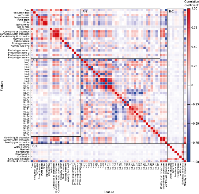
Fig. 1. Feature correlation analysis (No.0-No.32 are abstract features of category and numerical features after PCA dimension reduction). |
2.4. Division of oil well production histories
During the oil production history for over 60 years, there are significant stages of oil production changing tendency. To effectively grasp the characteristics of single well production change during different stages, it is necessary to divide well production history into different stages, and build the model for different stages separately. In this study, an algorithm was proposed to automatically divide the production history of single wells according to the water cut in oil wells. fw<30%, 30%≤fw<60%, 60%≤fw≤ 80%, fw>80% correspond to low, medium, high and ultrahigh water cut stages respectively (Fig. 2 ). Since water cut data is discontinuous or abrupt, but the production stages are relatively continuous, the water cut sequence of the training set should be stepwise processed before the stage division. We established 4 stage prediction models then integrated them. When predicting, give a production stage weight for each input month to determine the production stage of the target month, and then the corresponding stage model was used for prediction. The final prediction results of whole life cycle were obtained by splicing the prediction results of each stage.
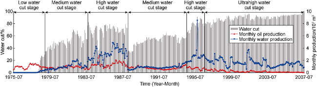
Fig. 2. Schematic diagram of production history division. |
In addition, the main control factors of monthly oil production during different production stages are different. Therefore, it is necessary to calculate the correlation coefficients during 4 production stages and selected the features with correlation coefficients greater than 0.2 or less than -0.2 to build input data sets respectively. The final input features of models of each stage are shown in Fig. 3 .
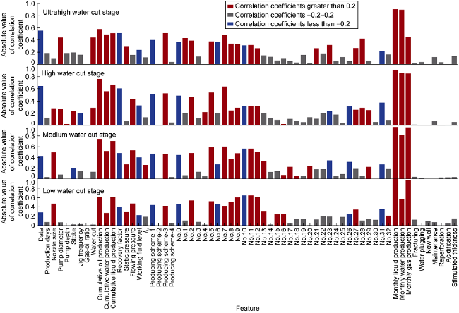
Fig. 3. Correlation coefficient between monthly oil production and influencing characteristics at each production stage. |
2.5. Time sliding window and data set division
Divide the data set taking well as unit: Data of 341 oil wells constitute the training set for model training, data of 43 oil wells constitute the validation set for hyperparameter optimization, and data of 42 oil wells constitute the testing set for the model testing. Specify the input step size and output step size and the input data are obtained by sliding time window. Constitute the input data and tags suitable for each model.
3. Model structure design and evaluation
3.1. Model structure design
According to the characteristics of single well production prediction task, such as multi-features, short input time step and small data volume, the TCN model was improved in 3 aspects: (1) Stack 1D convolutional layers with the kernel size of 1 before time convolutional layers to extract features; (2) Do not apply dilated convolution and residual connection, set the kernel size of the causal convolution layers as the input time step length. (3) Use the last time step in the output of the causal convolution layer for the final prediction. The structure of the improved TCN model is shown in Fig. 4 .
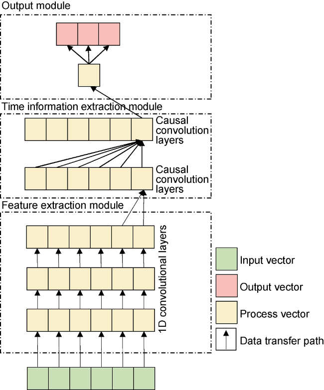
Fig. 4. Structure of improved TCN model. |
3.2. Hyperparameter design of sparrow search algorithm
Use SSA to optimize the hyperparameters of the models. The maximum number of iterations was 50, the number of producers was 20, the number of the sparrows which perceived the danger was 20, the safety threshold was 0.8, and the total number of sparrows was 100. Taking a model using 12 months’ data as input as an example, the hyperparameters of each layer of TCN model are shown in Table 1 .
Table 1. Optimal hyperparameters of the improved TCN model searched by SSA |
| Layers | Filters | Kernel size | Dilatation rate | Function |
|---|---|---|---|---|
| 1 | 46 | 1 | 1 | Feature extraction |
| 2 | 25 | 1 | 1 | Feature extraction |
| 3 | 10 | 1 | 1 | Feature extraction |
| 4 | 46 | 2 | 1 | Time information fusion |
| 5 | 125 | 12* | 1 | Time information fusion |
Note: *—A fixed model hyperparameters, representing by the input time step length in this study |
3.3. Design of comparative models
There were 11 production prediction models built based on 5 representative temporal sequence modeling networks for the adaptability of improved TCN model, as shown below: (1) The combined model of CNN and LSTM [13], CNN-LSTM; (2) The LSTM model; (3) LSTM model based on the seq2seq [14] supplemented with Luong Attention mechanism [15] for time dimension, named Attention-LSTM (T); (4) LSTM model supplemented with Temporal Pattern Attention [16] mechanism to realize the attention to different features, named Attention-LSTM (F); (5) LSTM model supplemented with both Luong Attention mechanism and Temporal Pattern Attention mechanism to realize the attention to different time steps as well as features, named Attention-LSTM (T&F); (6) Self-attention model for features [17⇓-19], named Self Attention (F); (7) Self-attention model for time dimension, named Self Attention (T); (8) Self-attention model both for time and features, named Self Attention (T&F); (9) LSTM model supplemented with a self-attention mechanism for features, named Self Attention-LSTM (F); (10) LSTM model supplemented with a self-attention mechanism for time steps, named Self Attention-LSTM (T); (11) LSTM model supplemented with a self-attention mechanism both for time steps and features, named Self Attention-LSTM (T&F). The hyperparameters of the comparison models were also optimized by SSA.
3.4. Design of the training set
In the training process, the model based on the seq2seq was used with the "Teacher Forcing" hybrid training strategy. Through the experiment, “Adagrad” was chosen as the model optimizer. The initial learning rate was set at 0.05. Callback function ReduceLROnPlateau was used to adapt the learning rate. To prevent overfitting, layer regularization was applied in the model, and training process was controlled by the callback function EarlyStop. It is worth noting that, to reduce the uncertainty caused by the potential randomness of the model, the model evaluation results in this paper are all from the average of 3 experiments under the same setting.
3.5. Model evaluation
Four evaluation metrics are used to evaluate the model: mean absolute error (MAE), mean absolute percentage error (MAPE), coefficient of multiple correlation (R2), root mean square error (RMSE), as shown in Eq. (3) to Eq. (6).
$ M A E=\frac{1}{N} \sum_{k=1}^{N}\left|q_{k}-\hat{q}_{k}\right|$
$ \text { MAPE }=\frac{1}{N} \sum_{k=1}^{N} \frac{\left|q_{k}-\hat{q}_{k}\right|}{q_{k}} \times 100 \%$
$ R^{2}=\frac{\sum_{k=1}^{N}\left(q_{k}-\bar{q}\right)^{2}-\sum_{k=1}^{N}\left(q_{k}-\hat{q}_{k}\right)^{2}}{\sum_{k=1}^{N}\left(q_{k}-\bar{q}\right)^{2}}$
$ R M S E=\sqrt{\frac{\sum_{k=1}^{N}\left(q_{k}-\hat{q}_{k}\right)^{2}}{N}}$
4. Application and discussion
4.1. Comparison of different algorithms
Taking input time step length of 12 months and output time step length of 3 months as an example, we used above 12 kinds of models to predict the production of 42 test wells. The results of the mean absolute error of the 13th month are shown in Table 2 . Notice that, the integrated models in Table 2 are model integrated by 4 stages models, and the single model is trained by whole data without stage division. Table 2 shows that the improved TCN model has the highest prediction accuracy, and the mean absolute error of the integrated one is 17.66 m3, 3.05 m3 lower than that of the single model.
Table 2. Comparison of the mean absolute errors in production at the 13th month predicted values of different models |
| Models | MAE of stage models/m3 | MAE of whole life prediction models/m3 | |||||
|---|---|---|---|---|---|---|---|
| Low water cut stage | Middle water cut stage | High water cut stage | Ultrahigh water cut stage | Integrated model | Single model | ||
| Improved TCN models | 23.22 | 17.93 | 13.15 | 19.53 | 17.66 | 20.71 | |
| Comparative models | CNN-LSTM | 30.86 | 18.89 | 19.84 | 21.44 | 21.39 | 21.60 |
| LSTM | 37.55 | 22.71 | 16.98 | 22.40 | 22.35 | 22.55 | |
| Attention-LSTM (T) | 65.26 | 31.31 | 38.95 | 28.13 | 35.72 | 30.20 | |
| Attention-LSTM (F) | 53.80 | 25.58 | 32.27 | 25.27 | 30.28 | 30.20 | |
| Attention-LSTM (T&F) | 75.77 | 38.00 | 42.78 | 31.95 | 40.79 | 40.71 | |
| Self-Attention (F) | 65.26 | 36.09 | 25.58 | 40.55 | 37.63 | 34.02 | |
| Self-Attention (T) | 131.19 | 61.89 | 33.22 | 49.15 | 55.12 | 33.06 | |
| Self-Attention (T&F) | 139.79 | 92.46 | 30.35 | 44.38 | 59.32 | 34.98 | |
| Self-Attention-LSTM (F) | 79.60 | 38.95 | 27.49 | 31.00 | 36.39 | 25.42 | |
| Self-Attention-LSTM (T) | 92.97 | 46.60 | 93.42 | 33.86 | 54.18 | 26.38 | |
| Self-Attention-LSTM (T&F) | 110.17 | 54.24 | 121.13 | 31.00 | 60.60 | 28.46 | |
Note: T—Attention mechanism for time; F—Attention mechanism for feature. |
Attention mechanism can improve the accuracy of time sequence prediction in machine translation and speech recognition[20⇓⇓-23]. In this study, we studied 9 models with attention mechanisms. The results show that the prediction precision is not good, representing the poor adaptability of attention mechanism to production prediction. (1) In fact, the production of a well in next moment does not heavily depend on the production of few moments before or its influencing factors, but the overall production change trend for a period. Also, the introduction of attention mechanism make the model give larger weights to some individual time steps, which interfering the production and the overall trend of its influencing factors in a period, leading to a decrease in the prediction accuracy of the model. (2) Furthermore, LSTM model already has the ability to analyze the production performance data of 12 months, the addition of attention mechanism greatly aggravates the training burden of the model, which is another possible reason for the low prediction accuracy of the model. (3) In addition, the introduction of attention mechanism means more parameters to be trained and more complex model structure. However, with the increase of model fitting capability, the weak noise in data set will be learned by model and mistake and overfitting will occur, which may reduce the prediction accuracy.
By comparing model performance during 4 different stages, it is found that the prediction accuracy of the low water cut stage models under all algorithms is the lowest. Because the that the low water cut stage is only a small part in the production process of oil wells, the number of samples is insufficient, and the model training is not sufficient.
4.2. Comparison of the correction methods for data padding
Randomly select 8 wells with relatively more missing dynamic data for comparison of data padding and correction. Table 3 lists the evaluation results with TCN models by using data processed by 4 different strategies: padded by the model proposed in this study, padded by average value without abnormal data correction, padded by interpolation with abnormal data correction and padded by average value with abnormal data correction. The 4 evaluation metrics all confirmed the effectiveness of the data padding and correction process in this paper, with the smallest average prediction error and the highest accuracy.
Table 3. Comparison of evaluation results with TCN models using samples processed by different filling and correction strategies |
| Data processing | MAE/m3 | MAPE/% | R2 | RMSE/m3 |
|---|---|---|---|---|
| Model proposed in this study | 23.83 | 5.16 | 0.99 | 63.57 |
| Average value without correction | 26.13 | 5.42 | 0.98 | 68.10 |
| Average value with correction | 25.72 | 5.32 | 0.98 | 69.25 |
| Interpolation with correction | 24.35 | 5.29 | 0.99 | 64.02 |
Note: Use the production data of 12 months to predict well production in the next 3 months; the data in table are evaluation results on the error of the predicted production at 13th month. |
4.3. Comparison of model input step length
Taking the single models as examples, we used TCN model and LSTM model to verify the influence of different input step length on prediction accuracy (Fig. 5 ). It is easy to see that the performance of TCN model is better than that of LSTM model when the input step length is short. However, with the increase of the input step length, the prediction error of TCN model increases significantly, while that of LSTM model is decreasing. Since the oil well production history has been divided into stages, and the average time span was reduced from 406 months to 103 months, if the long input step length was used, the number of samples would be very small, and mainly centralized in ultrahigh water cut stage, which would be limited in application. Fig. 5 shows that the prediction accuracy of TCN model is close in the time step range of 12-50 months. On the premise of ensuring the prediction accuracy of the model, a time step of 12 months was chosen to maximize the number of samples.
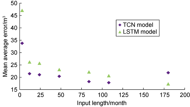
Fig. 5. Prediction results of TCN and LSTM models under different input step lengths. |
4.4. Analysis of model structure
4.4.1. Necessity of feature extraction by stacking 1D-convolutional layers
Table 4. Quantitative evaluation results of 3 predicted values by TCN models with and without feature extraction layers |
| Method | MAE/m3 | MAPE/% | R2 | RMSE/m3 |
|---|---|---|---|---|
| Without feature extraction layers (13) | 26.83 | 5.46 | 0.99 | 60.12 |
| Without feature extraction layers (14) | 39.67 | 6.98 | 0.97 | 86.58 |
| Without feature extraction layers (15) | 52.77 | 11.23 | 0.95 | 112.69 |
| With feature extraction layers (13) | 20.71 | 4.96 | 0.99 | 53.57 |
| With feature extraction layers (14) | 35.80 | 6.31 | 0.97 | 84.31 |
| With feature extraction layers (15) | 49.94 | 10.05 | 0.95 | 111.07 |
Note: Use 12 months production data to predict monthly well production in the next 3 months. (13), (14) and (15) are the predicted productions in 13th month, 14th month and 15th month respectively. |
4.4.2. Selection of the output from the causal convolution layer
Causal convolution layers have the same output time step length as the input layer. Whether all the outputs used for the final prediction or some selected outputs as the input of the next layer has a great influence on the prediction accuracy of the TCN model. We compared the prediction results under 5 conditions of using the full outputs, the outputs of the last 1 month, the outputs of the last 2 months, the outputs of the last 6 months, and the outputs of the last 10 months. The results showed that using full outputs would reduce the prediction accuracy of the model (Table 5 ). The last output has covered the inputs of preceding sequences, which is enough to complete the prediction.
Table 5. Effects of different output selection of the causal convolution layer on model prediction results |
| Output | MAE/m3 | MAPE/% | R2 | RMSE/m3 |
|---|---|---|---|---|
| Full outputs | 20.71 | 4.96 | 0.99 | 53.57 |
| The last 1 month | 20.81 | 4.97 | 0.99 | 53.59 |
| The last 2 months | 23.35 | 5.14 | 0.99 | 57.47 |
| The last 6 months | 24.12 | 5.28 | 0.99 | 57.53 |
| The last 10 months | 24.83 | 5.31 | 0.99 | 57.62 |
Note: Use the data of 12 months to predict monthly well production in the next 3 months. |
4.4.3. Selection of activation function
Bai et al.[11] proposed that adding generic residual module, regularization and activation function to the basic TCN architecture can improve the performance. To realize the nonlinear fitting capability of the model, the activation function was added in the 4th layer of the model. Comparison of TCN model prediction accuracy under different activation functions shows that in this paper, TCN model with softsign activation function outperforms other activation functions (Table 6 ). For this data set, the number of causal convolutional layers required to cover all inputs was not large, residual module was not used in the model. In addition, weight regularization is not required to prevent gradient disappearance. However, to prevent overfitting, layer regularization was applied after layer 3 and layer 5.
Table 6. Prediction results by TCN models with different activation functions |
| Activation function | MAE/m3 | MAPE/% | R2 | RMSE/m3 |
|---|---|---|---|---|
| softmax | 23.63 | 5.17 | 0.99 | 57.32 |
| sigmoid | 23.49 | 5.15 | 0.99 | 55.90 |
| softsign | 20.71 | 4.96 | 0.99 | 53.57 |
| relu | 28.87 | 5.73 | 0.98 | 64.18 |
| tanh | 23.13 | 5.12 | 0.99 | 58.10 |
Note: Use the data of 12 months to predict monthly well production in the next 3 months. |
4.5. Discussion of the model application results
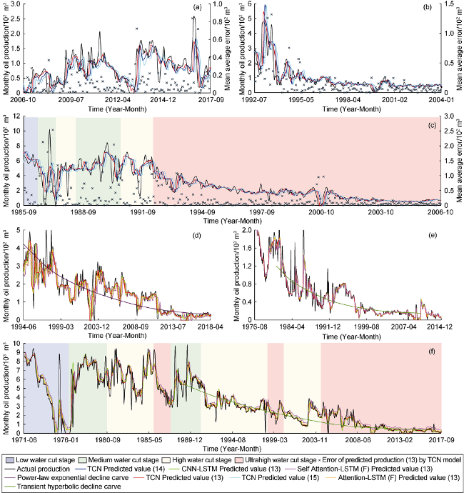
When forecasting oil well production, it is common to divide the production history of the oil well into two sections. The former is used as the training set and the latter is used as the testing set. In this study, full life cycle test was carried out to the prediction model. That is, all production data from 341 oil wells (training set) were used as training data to predict production of another 85 wells (validation set and testing set) until the production process was ended. The proposed model was used to predict oil production of 42 oil wells in the testing set. The prediction results of 6 wells were selected randomly for comparison, shown in Fig. 6 .
Fig. 6. Comparison of predicted and actual production of 6 randomly selected wells (predicted value (13) is the predicted production of 13th month by the model using historical data of the previous 12 months, predicted value (14) is the predicted production of 14th month, and predicted value (15) is the predicted production of the 15th month). (a) Comparison and error distribution between the actual production curve and the predicted production curve predicted by TCN of Well A; (b) Comparison and error distribution between the actual production curve and the predicted production curve predicted by TCN of Well B; (c) Comparison and error distribution between the actual production curve and the predicted production curve predicted by TCN of Well C; (d) Comparison between the actual production curve and the predicted production curve predicted by 5 different models of Well D; (e) Comparison between the actual production curve and the predicted production curve predicted by 5 different models of Well E; (f) Comparison between the actual production curve and the predicted production curve predicted by 5 different models of Well F. |
From Fig. 6 a to 6c, the prediction results of the model in 13th month, 14th month and 15th month are compared. In addition, we plotted the mean absolute error distribution of the prediction results at 13th month. Obviously, the prediction result of 13th month is the best, matching well with the real production curve. With the increase of the time interval, the gaps between the predicted production curves and the actual production curves increased obviously, and the hysteresis in inflection point gradually intensified. The error distribution shows that the larger error points usually occur at the peak/bottom tip of the curve. This is because the samples trained by the model are the output sequences processed by smoothing. Compared with the actual production data without smoothing, the change trend of the predicted values is relatively gentle.
To sum up, the model proposed in this paper can accomplish the prediction task of single well monthly production successfully. The prediction accuracy is higher than that of the traditional decline model and machine learning models such as LSTM with great application value.
5. Conclusions
A single well production prediction method based on temporal convolutional network model is proposed, which achieves efficient and accurate prediction of single well production. Random forest and principal component analysis, etc. are used for data padding and dimension reduction, which ensure the authenticity and completeness of data set. The sparrow search algorithm is used to search the optimal hyperparameters of proposed models, which improves the work efficiency, with high prediction accuracy. The production history of single wells are divided into 4 stages according to the water cut, namely low water cut stage, medium water cut stage, high water cut stage and ultrahigh water cut stage. The stage prediction model is developed separately, and then integrated to complete the full life cycle production prediction of individual well. The analysis and case results show that compared with other 11 kinds of time sequence models, the improved TCN model has better prediction performance. For the prediction of production sequences with large data fluctuations and obvious periodical characteristics, the method of dividing stage and subsection modeling can effectively reduce the difficulty of model fitting, and improve the prediction accuracy.
Nomenclature
Di,j—the distance between oil well i and water injection well j, m;
fw—water cut, %;
i—serial number of oil well;
j—serial number of water injection well;
It,i—the influence degree of the oil well i by water injection well j at time t, m3/m;
nw,i—total number of water injection wells affecting oil well i;
N—sample number;
k—serial number of monthly oil production samples;
qk—actual monthly oil production, m3;
$\hat{q}_{k}$—predicted monthly oil production, m3;
$\bar{q}$—average of actual monthly oil production, m3;
t—time (year-month);
Wt,j—monthly injection volume of water injection well j at time t, m3;
xo,i—x-coordinate of oil well i, m;
xw,j—x-coordinate of water injection well j, m;
yo,i—y-coordinate of oil well i, m;
yw,j—y-coordinate of water injection well j, m.