

Introduction
Shale oil resources in China are abundant, with recoverable reserves up to (30-60)×108 t, and are the most strategic and realistic oil replacement resources [1]. However, it is common that the initial production of a single well after fracturing is low, the production decline is fast, and the recovery degree is low, so the benefit development is facing great challenges [2-3]. For example, the Permian Lucaogou Formation shale oil reservoir in Jimsar sag of the Junggar Basin, NW China is a typical continental thin interbedded shale oil reservoir with fast longitudinal lithology change, thin interbeds and developed laminae (or bedding) [4]. Learning artificial fracture propagation mechanism and proppant distribution characteristics in shale oil reservoirs of this type is of great significance for improving the adaptability of fracturing process parameters and realizing the overall production of multilayer sweet spots.
International scholars have carried out a great deal of research on hydraulic fracture geometry, the height of fracture propagation and the interaction between fracture and bedding/interface in multilayered formations[5⇓⇓⇓⇓⇓-11]. It is found that hydraulic fractures in multilayered strata may have several behaviors such as crossing, turning, termination or stepped propagation after encountering bedding (or interface), and vertical propagation is easily
restricted, and the overall geometry is uncertain [5⇓⇓-8]. In general, simple fractures are easy to form in vertical homogeneous rocks, while complex fractures are easy to form in thin interbeds, which are controlled by the difference of mechanical properties between layers, stress difference between layers and interface properties[9⇓-11]. When stratified shale (or sandstone) has laminae (or beddings), it usually has significant mechanical anisotropy and is prone to fracture under the action of high pressure fluid or induced stress. The influence of laminae (or beddings) on fracture height and overall fracture geometry is very significant [12-13]. However, the current research on artificial fracture propagation mechanism of continental shale oil reservoirs in China is relatively insufficient [14], which restricts the optimization of fracturing parameter design. Compared with conventional single fracture, fracturing fluid flow field in complex fracture system is more complex, and proppant distribution directly determines the effectiveness of post-fracture[15-16]. Laboratory simulation of proppant migration in fractures mainly adopts the method of pre-set constant fracture size and geometry, which cannot consider the influence of real-time changes of reservoir fracture geometry on proppant distribution [17-18]. However, proppant is usually not added in laboratory fracturing experiments, and the distribution mechanism of proppant and the effectiveness of fracture are unknown under in-situ stress conditions [19⇓⇓-22]. Therefore, it is necessary to further study the dynamic migration and distribution of proppant during fracturing.
In this paper, the downhole cores of shale oil reservoirs in the Lucaogou Formation of Jimsar sag are selected to carry out physical simulation experiments of small-size true triaxial sand-carrying fracturing. Based on CT technology, the layer crossing performance of artificial fractures and the vertical distribution of proppant under the condition of stratigraphic-lithologic sequence combination are comprehensively analyzed, and the improved method of fracturing parameters of shale oil reservoir is discussed.
1. Experiment design
1.1. Sample preparation
The core samples are taken from the full diameter core of 6 sections of Well J10X of Lucaogou Formation in Jimsar sag. The coring depth is 3450-3667 m, the core diameter is 10-11 cm, and the core length is 10-35 cm (Fig. 1 ). The lithology of Core R1 is argillaceous shale, Core R2 is dolomitic mudstone, Core R3 is dolomitic siltstone, Core R4 is silty mudstone, Core R5 is argillaceous siltstone, and Core R6 is calcareous mudstone. The laminae of cores R1, R2 and R3 are relatively developed, and the key rock mechanical parameters are shown in Table 1 (the test confining pressure is 35 MPa). The parameter values of the core samples in the direction parallel to lamina are quite different from those in the direction vertical to lamina, presenting significant anisotropy. The anisotropy coefficient of elastic modulus (the ratio of elastic modulus in direction of parallel to lamina to that in direction of vertical to lamina) is 1.14-1.38, and the anisotropy coefficient of tensile strength (the ratio of tensile strength in direction of parallel to lamina to that in direction of vertical to lamina) is 1.05-2.26.

Fig. 1. Full diameter cores of Well J10X. |
Table 1. Test data of rock mechanical parameters |
| Core No. | Lithology | Elastic modulus/GPa | Anisotropy coefficient of elastic modulus | Tensile strength/MPa | Anisotropy coefficient of tensile strength | ||||
|---|---|---|---|---|---|---|---|---|---|
| Parallel to lamina | Vertical to lamina | Average | Parallel to lamina | Vertical to lamina | Average | ||||
| R1 | Argillaceous shale | 13.9 | 10.1 | 12.0 | 1.376 | 5.4 | 6.6 | 6.0 | 1.222 |
| R2 | Dolomitic mudstone | 31.4 | 25.2 | 28.3 | 1.246 | 7.1 | 8.1 | 7.6 | 1.141 |
| R3 | Dolomitic siltstone | 40.2 | 31.8 | 36.0 | 1.264 | 9.5 | 11.9 | 10.7 | 1.253 |
| R4 | Silty mudstone | 30.3 | 26.7 | 28.5 | 1.135 | 11.0 | 11.5 | 11.2 | 1.045 |
| R5 | Argillaceous siltstone | 26.5 | 21.0 | 25.1 | 1.262 | 3.9 | 8.8 | 7.2 | 2.256 |
| R6 | Calcareous mudstone | 12.9 | 9.9 | 12.1 | 1.303 | 3.8 | 4.8 | 4.0 | 1.263 |
In order to investigate the layer crossing performance of hydraulic fractures and the distribution of proppant under different lithological combinations, the full diameter core was cut into thin plates along the radial direction, and the thin interbedded shale sample was formed with high-strength epoxy resin glue according to the real stratigraphic lithological sequence (Fig. 2 a). The lithology of the upper and lower adjacent layers is identical, with a thickness of 2 cm. The middle layer is the perforated layer, with a thickness of 6 cm. A total of 3 thin interbedded fracturing rock samples were prepared, in which cores R1, R3 and R5 were set as perforated layers, and cores R2, R4 and R6 were set as adjacent layers. In Sample 1#, the adjacent layer is dolomitic mudstone, the perforated layer is argillaceous shale, the elastic modulus difference between the adjacent layer and the perforated layer is 16.3 GPa, the tensile strength difference is 1.6 MPa, and the adjacent layer belongs to a high-strength barrier layer. In Sample 2#, the adjacent layer is silty mudstone, and the perforated layer is dolomitic siltstone. The elastic modulus difference between the adjacent layer and the perforated layer is -7.5 GPa, the tensile strength difference is 0.5 MPa, and the strength of the adjacent layer is relatively low. In Sample 3#, the adjacent layer is calcareous mudstone, and the perforated layer is argillaceous siltstone. The elastic modulus difference between the adjacent layer and the perforated layer is -13.0 GPa, and the tensile strength difference is -3.2 MPa. The strength of the adjacent layer is low.
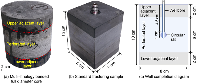
Fig. 2. Lithology combination sample preparation and well completion diagram. |
Thin-interbedded full diameter core was cut into 8 cm × 8 cm × 10 cm cuboid sample (Fig. 2 b). A hole with a diameter of 1.5 cm and a depth of 5.5 cm was drilled vertically at the center of the square plane to simulate a vertical well. A vertical circular cut (slit) with a radius of 0.2-0.3 cm was etched along the radial direction at the bottom of the wellbore to simulate perforation. A steel pipe with an outer diameter of 1.2 cm and a length of 5.0 cm was lowered to a position 1.0 cm from the bottom of the bottom hole to simulate a casing and the wellbore was cemented with the high-strength epoxy resin glue (Fig. 2 c). During the experiment, fracturing fluid and proppant were pumped into the wellbore, and the hydraulic fracture was induced to start at the circular cut after the high pressure was established.
1.2. Experimental equipment and steps
A small-scale true triaxial sanding-fracturing integrated simulation device was used in the experiment [19]. At present, the fracturing pumping rate of the shale oil horizontal well in Jimsar is 14-18 m3/min, and the number of clusters is 6-8. There is a difference in pumping rate between the initial fracturing stage and the main fracturing stage. It should be noted the maximum pumping rate of a single cluster is 3 m3/min, and the viscosity of fracturing fluid is 50-70 mPa·s (variable viscosity slick-water system). The main injection parameters in the experiments are calculated according to the similarity criterion [23⇓⇓-26] (Eq. (1) and Eq. (2)) in order to simulate the propagation process of viscous dominant fracture in the field. Considering that the characteristic radius of reservoir fracture propagation is about 18.00 m (i.e. the estimated fracture half height) while the characteristic radius of experimental fracture propagation is only 0.05 m (half of sample length), the maximum calculated experimental pumping rate is 50 mL/min, and the fracturing fluid viscosity is 100 mPa·s. The calculation results of field and indoor experimental parameters are shown in Table 2 .
$ \mu_{\mathrm{l}}=\alpha \mu_{\mathrm{f}}\left[\frac{t_{\max, \mathrm{l}}}{t_{\max, \mathrm{f}}}\left(\frac{Q_{\mathrm{f}}}{Q_{\mathrm{l}}}\right)^{3 / 2}\left(\frac{E_{\mathrm{f}}^{\prime}}{E_{\mathrm{l}}^{\prime}}\right)^{13 / 2}\left(\frac{K_{\mathrm{l}}^{\prime}}{K_{\mathrm{f}}^{\prime}}\right)^{9}\right]^{2 / 5}$
$ t_{\max }=\frac{R^{5 / 2} K^{\prime}}{Q E^{\prime}}$
Table 2. Main fracturing parameters of fracturing test |
| Fracturing parameter | Elastic modulus/ GPa | Fracture toughness/ (MPa·m1/2) | Characteristic radius of fracture/m | Single cluster pumping rate/(m3·min-1) | Fracturing fluid viscosity/(mPa·s) |
|---|---|---|---|---|---|
| Field | 24.2 | 3.60 | 18.00 | 3.000 00 | 50-70 |
| Experiment | 12.0-36.0 | 1.54 | 0.05 | 0.000 05 | 100 |
Limited by the equipment performance, the experimental stress parameters are set according to the relative value of reservoir stress. The field horizontal principal stress difference is 13 MPa, and the vertical stress difference is 15 MPa at shale oil reservoir of Lucaogou Formation in Jimsar [4]. So the maximum horizontal principal stress, the minimum horizontal principal stress and the vertical stress of the experiment are 18, 5 and 20 MPa respectively. The proppant is acted by white quartz sand with particle size of 75 μm (200 mesh, "Type 200 proppant" for short) and 106-140 μm (120-140 mesh, "Type 1214 proppant" for short), and the sand concentration is 15-20 g/100 mL. The specific experimental schemes are shown in Table 3 .
Table 3. Fracturing simulation experiment schemes |
| Sample No. | Lithology combination (perforated layer + adjacent layer) | Pumping rate/ (mL·min-1) | Proppant type |
|---|---|---|---|
| 1# | R1+R2 | 20-50 | Type 200 |
| 2# | R3+R4 | 20-50 | Type 200, Type 1214 |
| 3# | R5+R6 | 5-50 | Type 200, Type 1214 |
Experimental steps: (1) Put the rock sample in the core chamber and load the minimum horizontal principal stress, the maximum horizontal principal stress and the vertical stress according to the above-mentioned parameters [19]. (2) Start the pumping system, inject the fracturing fluid mixed with fluorescent agent into the wellbore at a low pumping rate (5-20 mL/min), and record changes of wellhead pressure. After the rock breaks, the wellhead pressure will decrease rapidly, which corresponds to the end of pre-pad fluid injection stage. Then it is raised to a larger pumping rate (50 mL/min), and the sand outlet valve of the sand tank containing proppant is opened. After the proppant is mixed with the fracturing fluid, it enters the fracturing pipeline, which means the beginning of the sand-carrying fluid injection stage. Inject mixed mortar constantly, and don’t stop the pump until the wellhead pressure rises sharply and then drops. Type 200 proppant is used in the whole injection process of sand-carrying fluid to inspect the filling situations of small particle size proppant during the growth of lamina in Sample 1#. For samples 2# and 3#, Type 200 proppant is used for 120 s before the injection of sand-carrying fluid, and then Type 1214 proppant is used. The maximum cumulative liquid injection volume of a single group of experiments is 500 mL, and the maximum dosage of proppant is 50 g. (3) Scan the gray image of the sample by using the micron CT scanner, and reconstruct the core based on high-precision CT data. Combined with tracer distribution data and rock sample dissection results, comprehensively analyze and identify the fracture morphology and proppant distribution on the surface and inside of the rock sample.
Classify and process the gray image of the sample by using the VOLUME GRAPHICS STUDIO MAX software, analyze its structural and morphological characteristics (including fracture area, proppant volume, etc.), then build a three-dimensional digital core model, and calculate the complexity of fracture space by using the box-counting method [27-28]:
$ D_{\mathrm{f}}=\lim _{\delta \rightarrow 0} \frac{\log M}{\log (1 / \delta)}$
2. Morphological characteristics of artificial fractures
The perforated layer in Sample 1# is argillaceous shale, and its upper and lower adjacent layers are dolomitic mudstones. The artificial fractures were morphologically shaped as "丰" or "井" in the vertical direction (Fig. 3 ). The total fracture area was 38 010 mm2, in which the artificial fracture area and lamina fracture area accounted for 24.1% and 75.9% respectively, and the fracture complexity degree was about 2.48. The perforated layer in Sample 2# is dolomitic siltstone, and the upper and lower adjacent layers are silty mudstones. The overall vertical morphology of artificial fractures was similar to the shape of “〸” (Fig. 4 ). The total fracture area was 14 093 mm2, in which the artificial fracture area and laminar fracture area accounted for 58.7% and 41.3% respectively, and the fracture complexity degree was about 2.13. The perforated layer of Sample 3# is argillaceous siltstone, and its upper and lower adjacent layers are calcareous mudstones. Three branch fractures were generated on one side of the rock sample and crossed together on the other side (Fig. 5 ). The total area of fractures was 17 475 mm2, in which the artificial fracture area and laminar fracture area accounted for 96.4% and 3.6% respectively, indicating that artificial fractures were dominant and the fracture complexity degree was about 2.28. The results show that the artificial fractures are the most complicated in argillaceous shale, relatively complicated in argillaceous siltstone, and relatively simple in dolomitic siltstone.
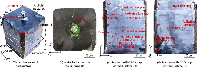
Fig. 3. Artificial fractures morphology on the surface of Sample 1#. |
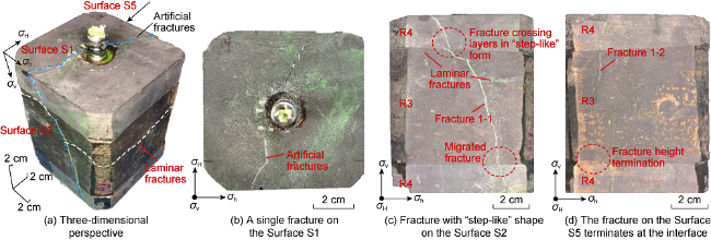
Fig. 4. Artificial fractures morphology on the surface of Sample 2#. |
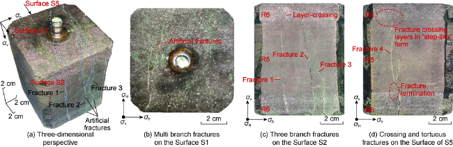
Fig. 5. Artificial fractures morphology on the surface of Sample 3#. |
2.1. Activated laminas and layer-crossing
There are great differences in activated laminae in different lithology samples. One artificial fracture (Fracture 1) was formed on one side of the perforated layer of Sample 1#, and two artificial fractures (Fracture 1 and Fracture 2) were formed on the other side. Artificial fractures activated multiple laminae in the upper and lower parts of the perforated layer, in which the top of Fracture 1 penetrated the entire upper adjacent layer, the top of Fracture 2 terminated at the lithologic interface and migrated at the thin interlayer interface in the lower part of the perforated layer (Fig. 6 a). And the bottom of both fractures terminated at a lamina near the lithologic interface in the lower adjacent layer (Fig. 3 ). In the perforated layer of Sample 2#, an artificial fracture was formed running through the upper and lower adjacent layers, and induced the partial activation of many laminae in the upper part of the perforated layer. The artificial fractures all deviated horizontally after encountering the activated laminae and lithologic interfaces, resulting in the “step-like” propagation of fractures in the vertical direction (Fig. 4 ). Three closely-spaced hydraulic fractures ran through the upper and lower adjacent layers as a whole were generated in the perforated layer of Sample 3#, but some branch fractures terminated or migrated through the interlayer interface (Fig. 5 ).
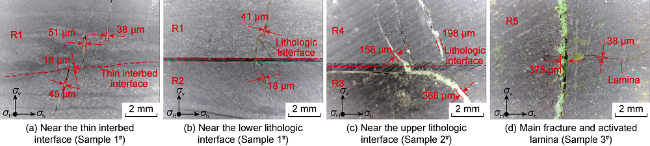
Fig. 6. The local morphology and width variation of artificial fractures on the sample surface. |
Under experimental conditions, the adjacent layer with high mechanical strength (Sample 1#), lower mechanical strength (Sample 2#) and low mechanical strength (Sample 3#) had no obvious hindering effect on the vertical propagation of fractures, and only the local fracture propagation in the vertical direction terminated at the lithologic interfaces. What’s more, the experimental results also show that the use of high viscosity fracturing fluid (100 mPa·s) is conducive to the layer-crossing propagation of near-wellbore artificial fracture.
2.2. Vertical fracture width variation and proppant distribution
Vertically, artificial fracture widths varied greatly from perforated layers to adjacent layers, typically narrowing at laminae and interlayer interfaces (Fig. 6 ), which significantly affected proppant transportation and distribution.
2.2.1. Combination of argillaceous shale and dolomitic mudstone
Statistical fracture width of Fracture 1 in Sample 1# along the fracture height direction is shown in Fig. 7 . In Sample 1#, the average fracture width of artificial fractures near the perforating position (the coordinate of fracture height direction z=0) is about 69.5 μm (the mean fracture width of two wings). In the process of upward fracture propagation, the fracture width gradually increased first and then decreased, and the fracture width of the two wings (fractures 1-1 and 1-2) reached the maximum value near z=2.5 cm, with the width of fractures 1-1 and 1-2 reaching 215.0 μm and 175.0 μm, respectively. Besides, the fracture width decreased rapidly after the artificial fractures crossed the upper lithologic interface and entered the upper adjacent layer (R2). The average fracture width of Fracture 1-1 was 173.8 μm, and that of Fracture 1-2 was 147.4 μm in the upper adjacent layer. In the process of downward fracture propagation, the overall fracture width tended to narrow. The fracture width decreased rapidly, from 34 μm to 21 μm at Fracture 1-1 and from 37 μm to 19 μm at Fracture 1-2 due to the occurrence of thin interbed in the vicinity of z=-1.5 cm. The fracture width was further narrowed after entering the lower adjacent layer, and the average width of fractures 1-1 and 1-2 was only 14.0 μm and 13.0 μm, respectively. In addition, in the vicinity of z=0, z=2 and z=-4 cm, there were laminar fractures with width of 57, 45, and 18 μm, which were much smaller than the width of vertical artificial fractures.
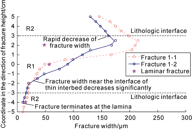
Fig. 7. Statistical fracture width of Sample 1# along the vertical direction. |
The total fracture volume in Sample 1# was 3877.5 mm3, with a proppant filling volume of 481.6 mm3, accounting for 12.4%. The proppant was mainly accumulated in the upper and middle part of the sample (z is -1.0-4.0 cm), which was the artificial fracture with larger fracture width. However, there was also a small amount of proppant in the activated laminar fracture near the main fracture in the lower part (Fig. 8 ). At the same time, most of the proppant was transported and distributed in the perforated layer, with only a small amount entering the upper adjacent layer. The height of artificial fracture and propped fracture were 9.0 cm and 5.2 cm, respectively, accounting for 57.8%; and the length of artificial fracture and propped fracture were 8.0 cm and 6.1 cm, respectively, accounting for 76.3%.
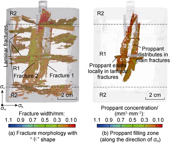
Fig. 8. Three-dimensional reconstruction of artificial fracture morphology in Sample 1#. |
2.2.2. Combination of dolomitic siltstone and silty mudstone
Statistical fracture width of Sample 2# is shown in Fig. 9 . It is shown that the average fracture width of the two wings of the artificial fracture varied greatly in the vicinity of the perforation position (z=0), with the average fracture width of 525.0 μm and 115.0 μm for fractures 1-1 and 1-2. In the process of upward fracture propagation, the fracture width gradually increased first and then decreased, and the fracture width of the two wings reached the maximum value near z=1.5 cm, with the fracture width of 537.0 μm for Fracture 1-1 and 291.0 μm for fracture 1-2. The fracture width decreased rapidly when the artificial fracture entered the upper adjacent layer (R4) by penetrating the upper lithologic interface, and the average fracture width of fractures 1-1 and 1-2 in the upper adjacent layer were 330.8 μm and 173.8 μm, respectively. In the process of downward fracture propagation, the overall fracture width tended to narrow, especially after entering the lower adjacent layer, and the average fracture width of fractures 1-1 and 1-2 in the adjacent layer were 226.2 μm and 13.6 μm, respectively. In addition, there was an activated laminar fracture near z=0.5 cm with a width of 114.0 μm, which was much smaller than the width of vertical artificial fracture.
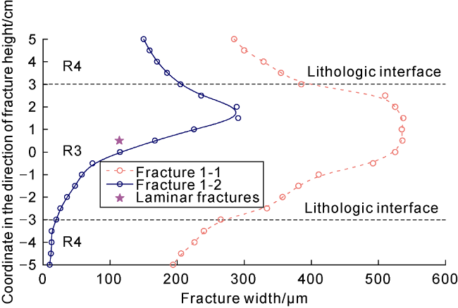
Fig. 9. Statistical fracture width of Sample 2# along the vertical direction. |
The total fracture volume in Sample 2# was 2339.4 mm3, of which the proppant filling volume was 923.1 mm3, accounting for 39.5%. The proppant was mainly concentrated in the Fracture 1-1 with larger width in the middle and upper part of the sample (z=-1.0-4.0 cm), and there was almost no proppant in the laminar fracture (Fig. 10 ). As a result, only a small amount of proppant was transported into the upper adjacent layer, while there was almost no proppant in the lower adjacent layer. The height of artificial fracture and propped fracture were 10.0 cm and 5.2 cm, respectively, accounting for 52.0%, and the length of artificial fracture and propped fracture were 8.0 cm and 5.3 cm, respectively, accounting for 66.3%.
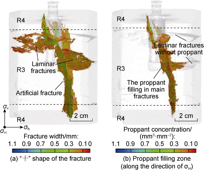
Fig. 10. Three-dimensional reconstruction of artificial fracture morphology in sample 2#. |
2.2.3. Combination of argillaceous siltstone and calcareous mudstone
Multi-branch vertical artificial fractures were formed in Sample 3#, so the variation of fracture width vertically was complicated (Fig. 11 ). From the upper adjacent layer, perforated layer to the lower adjacent layer, the fracture width increased gradually on the whole, but fluctuated locally. The three closely-spaced branch fractures (Fractures 1, 2 and 3) formed on one side of the sample were significantly narrower than the single fracture (fracture 4) formed on the other side. The average width of the three branch fractures near the perforated position (z=0) was 137.3 μm, while that of Fracture 4 was 416.0 μm. The average width of the three branch fractures reached the maximum value of 244.0 μm near z=-3.0 cm, while the width of Fracture 4 reached the maximum value of 425.0 μm near z=-1.0 cm. In the upper adjacent layer, the average width of three branch fractures and the width of Fracture 4 were 56.7 μm and 161.4 μm, respectively. In the lower adjacent layer, the average width of three branch fractures and the width of Fracture 4 were 265.8 μm and 527.0 μm, respectively.
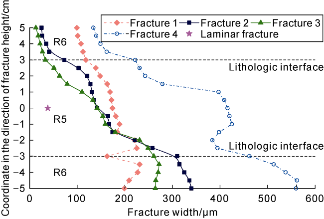
Fig. 11. Statistical fracture width of Sample 3# along the vertical direction. |
The total fracture volume in Sample 3# was 4378.3 mm3, with a proppant filling volume of 777.7 mm3, accounting for 17.8%. The proppant was mainly distributed in the Fracture 4, and there was only a small amount of proppant in the three branch fractures (Fig. 12 ). In addition, the proppant was concentrated mainly in artificial fractures near the perforated layer, and did not migrate to the upper adjacent layer. The height of artificial fracture and propped fracture were 10.0 cm and 4.7 cm, accounting for 47.0%, and the length of artificial fracture and propped fracture were 8.0 cm and 5.5 cm, accounting for 68.9%.
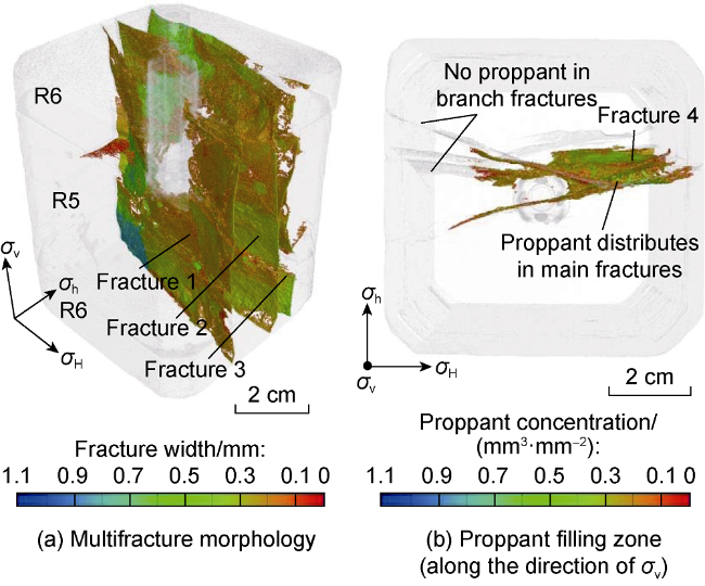
Fig. 12. Three-dimensional reconstruction of artificial fracture morphology in Sample 3#. |
Based on the morphology and width of hydraulic fractures and the proppant distribution, it is indicated that the limit width to enter hydraulic fracture was about 200 μm for Type 200 proppant and about 350 μm for Type 1214 proppant. The limit width of proppant entering the fracture was about 2.7 times the proppant particle size, which was slightly larger than the 2.5 times obtained by Cipolla et al. [29] and slightly smaller than the 3 times obtained by Gruesbeck [30].
3. Fracturing operation curve
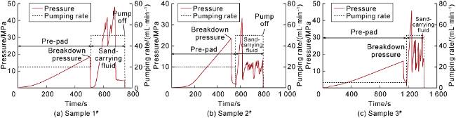
The fracturing curve characteristics of the three samples differ greatly (Fig. 13 ). (1) For Sample 1#, the breakdown pressure reached 18.3 MPa at 505 s with the pumping rate of 20 mL/min during the pre-pad injection stage of 0-512 s (Fig. 13 a), and the pressure rise rate before fracturing was 0.045 MPa/s. During the injection of sand-carrying fluid from 513 s to 749 s, the pumping rate was increased to 50 mL/min, and Type 200 proppant was used in the whole process. The pumping pressure rose rapidly in the initial stage of construction, and then fluctuated greatly twice due to the transportation and accumulation of proppant in the fracture. This indicated the possibility of proppant screen-out, resulting in a maximum pressure of 48.1 MPa (679 s), which was much higher than the breakdown pressure. The pumping pressure decreased rapidly with the increase of artificial fracture width, and the injection was stopped at 749 s. (2) For Sample 2#, the breakdown pressure reached 23.6 MPa at 521 s with the pumping rate of 20 mL/min during the pre-pad injection stage of 0-559 s (Fig. 13 b), and the pressure rise rate before breakdown was 0.063 MPa/s. During the injection of sand-carrying fluid from 560 s to 801 s, the injection rate was increased to 50 mL/min. In this stage, Type 200 proppant was added during 560-680 s and Type 1214 proppant was added during 681-801 s. The pumping pressure rose rapidly after 560 s, and reached the maximum value of 33.1 MPa at 617 s, which was higher than the breakdown pressure. Then the pumping pressure dropped rapidly and remained at about 10.2 MPa, and the injection was stopped at 801 s. (3) For Sample 3#, the breakdown pressure reached 15.9 MPa at 1131 s with the pumping rate of 5 mL/min during the pre-pad injection stage of 0-1173 s (Fig. 13 c), and the pressure rise rate before breakdown was only 0.017 MPa/s, lower than that of samples 1# and 2#. During the injection of sand-carrying fluid from 1174 s to 1418 s, the pumping rate was increased to 50 mL/min. In this stage, Type 200 proppant was added during 1174-1296 s and Type 1214 proppant was added during 1297-1418 s. The pumping pressure rose rapidly and reached the maximum value of 45.9 MPa at 1248 s, which was higher than the breakdown pressure. Then the pumping pressure dropped rapidly and fluctuated within 9.2-32.3 MPa, and the injection was stopped at 1418 s.
Fig. 13. Fracturing operation curve of the rock samples. |
It is indicated by comparing the pressure curves of three samples that the breakdown pressure of Sample 2# is the highest due to the maximum rock strength (E=36.0 GPa, T=10.7 MPa) in the perforated layer. The pressure is overall lower and stable during the injection of sand-carrying fluid, so the main fracture is initiated sufficiently with greater fracture width, and the sanding is overall successful. The breakdown pressure of Sample 1# is lower due to the lowest rock strength (E=12.0 GPa, T= 6.0 MPa) in the perforated layer, more developed laminae, and great fracturing fluid loss. Furthermore, the initiation of main fracture in Sample 1# was not sufficient, resulting in smaller fracture width, higher pressure during the injection of sand-carrying fluid and obvious proppant plug phenomenon. The rock strength of Sample 3# in the perforated layer was medium (E=25.1 GPa, T=7.2 MPa), but the breakdown pressure was the lowest. In addition, the fracture initiation was not sufficient due to the low pumping rate in the pre-pad injection stage, resulting in the formation of many fractures of small width during the injection of sand-carrying fluid. As a result, the pumping pressure is higher and fluctuated frequently, and it’s difficult to carry out sanding.
4. Conclusions
In thin-interbedded shale oil reservoirs, interlayer rock mechanical differences and interfaces near wellbore have no obvious shielding effect on fracture height propagation, but have a significant effect on the distribution of fracture width in the direction of fracture height. Hydraulic fractures tend to propagate through layers in the form of "step-like", and the fracture width is narrow at the interface deflection, which hinders vertical migration of proppant and causes poor layer crossing performance. For example, lamina is developed in shale, so it is easy to form "丰" or "井" shaped fractures.
If the perforated interval has large rock strength and high breakdown pressure, the initiation of main fracture is sufficient, the fracture width is large and consequently the overall sanding effect is good. In contrast, if the perforated interval has low rock strength and developed laminae, the fracturing fluid filtration loss is large, the breakdown pressure is low, the initiation of main fracture is not sufficient, the fracture width is small, and consequently sand plugging is easy to occur.
Proppant is mainly concentrated in the main hydraulic fractures with large width near the perforated layer, and activated laminae, branch fractures and fractures in adjacent layers contain only a small amount of (or zero) proppant. The proppant is placed in a limited range on the whole. The limit width of fracture that proppant can enter is about 2.7 times the proppant particle size.
Nomenclature
Df—degree of fracture space complexity, dimensionless;
E—elastic modulus of rock, GPa;
E°—plane strain elastic modulus, GPa;
K°—modified fracture toughness, MPa·m1/2;
M—the minimum number of cubes (boxes) required to cover the target object with diameter δ;
Q—pumping rate, m3/min;
R—fracture characteristic radius, m;
t—fracture propagation time, s;
T—tensile strength, Mpa;
z—fracture height coordinates, cm;
α—similarity coefficient, which is about 0.85, dimensionless;
δ—diameter of the cube (box), m;
μ—fracturing fluid viscosity, mPa·s;
σh—minimum horizontal principal stress, MPa;
σH—maximum horizontal principal stress, MPa;
σv—vertical stress, MPa.
Subscripts:
f—field parameter;
l—laboratory parameter;
max—maximum.