

Introduction
Reservoir simulation is traditionally required as a decision-making tool in reservoir management studies, as it provides the physical representation of static characteristics and dynamic behaviour of a hydrocarbon reservoir, while considering a large number of known uncertainties. The history matched model is essential for reservoir management to assess different strategies maximizing hydrocarbon recovery. History matching is the model calibration exercise, which relies on the fact that if a model can accurately reproduce the production history or observed data, it will be useful to predict the future performance of the reservoir. One of the main challenges for reservoir engineers during the history matching process is to reproduce detailed information about the fluid displacement in the porous media in order to identify the time of water breakthrough for each well and each pay zone in a production well. On that topic, Benlacheheb et al. [1] highlighted the advantages of incorporating additional monitoring data as part of the history matching process to allow more detailed outcome related to vertical heterogeneity of reservoir properties in the validated model. This research aims to develop a complementary methodology to improve the results obtained from the history matching process by incorporating binary saturations logs as a part of the evaluation parameters. The proposed methodology leads to a more robust and reliable reservoir model.
The novelty of the methodology proposed in this paper lies in its flexibility to include new evaluation parameters independent of the type of data. Besides, the methodology also provides a simplification of the matching responses by transforming the original format into binary output, which opens the possibility to use more complex frameworks to accelerate the matching process such as machine learning.
1. Theoretical basis
1.1 Objective functions
The history matching quality of a model is often expressed in terms of its global objective function. The objective function is a mathematical function that allows a measure of the misfit between simulated and observed data [2]. Most of the existing formulations can be written as a function of a point-by-point difference between simulated and historical data.
In a conventional history matching process, all reservoir data is gathered to create a 3D model through the reservoir characterisation process. Then, by using dynamic simulation and the observed data, the model is used to predict historical results. Finally, simulated results are compared to the observed data using the objective function to determine the history matching quality of the model. More holistic approaches have been introduced into geomodelling processes by unlocking the potential of assessing a significant number of possible combinations of inputs used to create the 3D model, and creating a wide range of alternative solutions [3-4]. These alternative solutions are commonly described as representative group of models. The final representative group of models are selected from a bigger equally probable ensemble which is derived from the combination of all related uncertainties in an uncertainty analysis. The selection of the representative group of models is based on their history matching quality. The rationale of these original approaches is based on the nature of the history matching as an inverse problem optimisation which means that there is no unique solution to the problem and hence different sets of inputs could lead to almost the same outcome.
The incorporation of the geologist’s interpretation data as part of the whole process provides the results with more information about the most representative reservoir models and uncertainties about static reservoir data[5-6]. The selection of the different objective functions used for the evaluation of model’s performance and efficiency was reviewed by Mata-Lima [2]. Further findings from published data show that root mean squared error (RMSE) as well as mean of the deviations (AE) are the most widely used in history matching, considering the linear nature of the parameters commonly used in the process. However, many of these deviation-based statistics differ from each other in the way that differences between observed and simulated results are evaluated.
1.2. Limitation of conventional objective function calculations
In conventional history matching workflows, the objective function is commonly calculated using well level production data such as production rates (oil, gas, water, or total liquid rates), gauge pressures and production ratios such as well water cut. It is well known that for any model-built process, the more the number of key performance indicators (KPIs) the model managed to represent, the better the quality of the model. Hence, matching a reservoir model using only limited data may not be enough to define a satisfactory representation of the reservoir in order to predict its future performance [7]. One of the main challenges of using well production data to validate the models is to accurately capture the correct saturation changes in individual producing zones in commingled production wells. Frequent practice evokes two methods to measure near-wellbore water saturation changes, that is, saturation logs and 4D seismic. The use of 4D seismic technology has positively contributed to a better interpretation of fluid displacement [8-9]. However, this technology can lead to some difficulties which require additional algorithms and statistical analysis to predict fluid saturations. Besides, 4D seismic data is not always available and has additional economic implications on the budget. On the other hand, saturation logs are commonly obtained during regular surveillance interventions.
1.3. Classification metrics
Several classification techniques have been applied in different fields of sciences depending on the nature of the problem and the classification output (binary or multi-class) [10].
1.3.1 Confusion matrix
The confusion matrix (CM) is defined as a table that allows the user to analyze results and performance of a specific algorithm which classifies data. The confusion matrix is one of the most common tools used to assess binary classifiers. A CM contains information about actual and predicted classifications done by a classification system [11]. The performance of such systems is commonly evaluated using the data in the matrix. Fig. 1 shows an example of the confusion matrix for a two-class classifier.
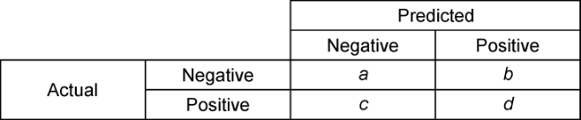
Fig. 1. The confusion matrix for two-class classification problem. a—the number of correct predictions for a negative instance or true negatives (TN); b—the number of incorrect predictions for the negative instance or False Positives (FP); c—the number of incorrect predictions for a positive instance or False Negatives (FN); d—the number of correct predictions for the positive instance or True Positives (TP). |
A wide portfolio of metrics used for binary classification assessments can be found in the literature and most of these metrics are derived from the CM. However, many of these metrics can be only applied to specific problems due to their biases and limitations as noted by Powers [12]. Fig. 1 summarizes the applicability and limitations of some of the more widely used binary metrics.
1.3.2. The Matthews correlation coefficient (MCC)
The MCC is a confusion matrix derived metric which was introduced by Brian W. Matthews in 1975 when comparing chemical structures [13]. MCC represents the correlation between the observed and predicted classifications with the advantage of overcoming problems generated for cases with imbalanced data by comparison with different confusion matrix metrics [14]. As others confusion matrix metrics, MCC can be calculated using predicted instances of the confusion matrix (TP, TN, FP and FN).
The MCC outcomes goes from −1 to 1, where a coefficient 1 indicates a perfect prediction or perfect match, −1 represents total disagreement between prediction and true values, and zero means no better than a random prediction. MCC is the only binary classification metric that generates a high score only if the binary predictor is able to correctly predict most positive and negative data instances. According to previous statistical studies and data science applications [14], in most of the cases, MCC can provide more reliable statistical results than other imbalanced binary metrics such as F-measure and Accuracy.
Although the classification metrics defined in Table 1 have been widely applied for data science and engineering problems, there is not public evidence of their applicability as part of history matching objective functions.
Table 1. Metrics used for binary classification, adapted from Tharwat [10] |
| Binary Metric | Key features | Application | Formulae |
|---|---|---|---|
| Confusion Matrix (CM) | CM measures the correlation between the observed and predicted data as quality of a binary response (true/false), (positive/negative). | The CM allows the application of the different metrics to correlate the data. | |
| False Positive Rate (FPR) | FPR represents the proportion of positive cases that are incorrectly classified as positive from the total number of negative outcomes. | Also recognized as fallout and false alarm rate. This metric is not affected by imbalanced data. | |
| True Negative Rate (TNR) | TNR represents the proportion of negative cases that are properly identified as negative from the total number of negative outcomes. | It is also called specificity or inverse recall. This metric is less affected by imbalanced data. | |
| False Negative Rate (FNR) | FNR represents the proportion of negative cases that are incorrectly identified as negative from the total number of negative outcomes. | It is also called miss rate or inverse recall. This metric is less affected by imbalanced data. | |
| Precision (P) | Represents the ratio of correct predictions that are relevant. When the prediction is yes, how often is it correct? | It is also called “confidence” metric. It does not consider the number of true negatives. | |
| Recall (R) | Measure the accuracy on the positive class. Thus, when the correct prediction is yes, how often does it predict yes? | The metric is valuable to measure the real positive cases that are predicted. The metric is represented as a rate of discovery of positive classifiers. | |
| F-Measure (FM) | It is the ratio of metrics Precision/Recall. It is the harmonic mean of precision and recall metrics. | It considers the ratio of True Positives to the arithmetic mean of predicted positives and real positives. This metric is sensitive to changes in the class distribution. | |
| Accuracy (A) | Represents the ratio between correct predictions to all predictions. The best value is 1 and the worst value is 0. | The metric is not reliable for imbalanced data. It can provide an overoptimistic estimation of the classifier. | |
| Matthew’s correlation coefficient (MCC) | Represents the relation between the observed and predicted classes. | The outcome ranges from +1 to -1, +1 represents a perfect prediction and -1 total disagreement. The metric is sensitive to imbalance data. | Where: A=TP*TN B=FP*FN C=TP+FP D=TP+FN E=TN+FP F=TN+FN |
2. Methodology
In order to evaluate the advantages and quality enhancement of the proposed methodology compared with a conventional history matching whose objective function only uses the production rate, a semi-synthetic geological model developed by UNISIM-M [15] was used in combination with a benchmarking workflow.
2.1. Benchmarking the proposed methodology
To benchmark the proposed methodology, a modified “Big Loop” workflow was used (Fig. 2 ). This benchmarking workflow differs from the original presented by Kumar [3] as it only uses the first iteration of the loop to generate the ensemble of models and it does not iterate to improve the history matching quality of the ensembles.
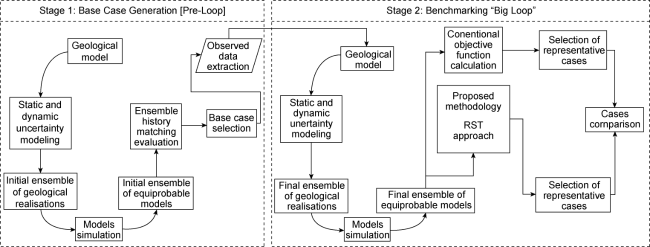
Fig. 2. Modified “Big Loop” workflow. |
The modified workflow is divided in two stages: Stage 1, or pre-loop, which is used to generate a base or control case to represent the real reservoir outcomes or “observed” data. In the Stage 2, a final ensemble of models is created from the base case. The final ensemble of model is later used to benchmark the proposed methodology by comparing the performance of both, conventional and enhanced proposed approaches in a model selection assessment.
Stage 1 includes the base reservoir model building (or observed data case) using all available data. Geological and dynamic inputs are analysed and included in the workflow. Variables and ranges of uncertainty are defined and analysed. The initial ensemble of models is generated as result of an uncertainty analysis loop using MonteCarlo permutation in combination with a Latin-hypercube sampling method. After the base case is generated, key producers are identified to evaluate the methodology. In real applications, this step will depend on the data available in terms of number of saturation logs per well. For the purpose of this study, all producer wells existing in the model were considered, and one reservoir saturation (RST) logs per year per well were generated.
To generate the final ensemble of models in Stage 2, a second uncertainty analysis loop is performed using the same inputs and variables defined in the previous stage. The difference between stages 1 and 2 uncertainty analyses is that the observed data used in Stage 2 correspond to the simulation data of the base case selected in Stage 1. After the final ensemble of models is generated, both, traditional and proposed methodologies are used to select the best history matching models from the ensemble. To select the models, the traditional approach uses an objective function calculation based on producer’s water cut. The proposed RST approach methodology uses binary RST logs and a confusion matrix metric to select the group of best matching cases. To assess the history matching quality of individual cases in each group, different key performance indicators (KPIs) such as the well and layer production rates are used to compare the selected cases against the base case.
2.2. Proposed RST approach methodology
The proposed methodology is an add-in module that can be used as an additional validation step in any history matching process as indicated previously in Fig. 2 . By incorporating reservoir water saturation change, which is derived from cased hole saturation logs, into the history matching process; the proposed methodology improved the fitting precision in terms of matching water saturation changes around producers. The new proposed methodology for enhanced history matching process using RST logs is represented in more details in Fig. 3 and each step is explained on this section.
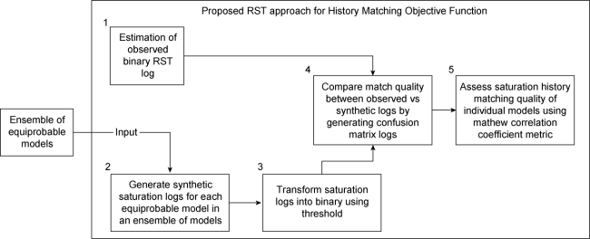
Fig. 3. Methodology proposed for enhanced history matching process using RST logs. |
2.2.1. Estimation of observed binary interpretation of reservoir saturation logs
The location and movement of the waterfront or sweep for each producer well is a key uncertainty in understanding and modelling the behaviour of an oil reservoir through production. Water saturation changes in the reservoir can be monitored by acquiring cased hole saturation logs. The standard interpretation approach for estimating cased hole saturation changes is based on log analysis of the cased hole log data. The process requires the use of a formation evaluation model that includes rock and fluid properties to interpret the log responses, and additional parameters to model the borehole configuration. The purpose of this interpretation is to estimate the water saturation. The results obtained from this interpretation approach contain high uncertainty, as there are many unknown parameters in the formation evaluation model, and the data can be noisy, which represents some challenges in the use of this data as a history matching parameter.
The proposed approach overcomes some of the challenges associated with the use of saturations logs for history matching by creating an interpreted binary (yes/no) “sweep” flag that represents the break-through of the waterfront. Although this binary sweep interpretation approach is a simplification of the normal process, it can be a valid characterisation of the saturation in several ways. The simplification reduces the grade of uncertainty created to determine a specific saturation value which is usually well defined when the waterfront has arrived. Analysis of time-lapse saturation logs shows that for any specific depth interval, there is a single and appreciable change of water saturation from a lower initial value to a higher one, corresponding to the arrival of the waterfront. This large, one-time change in water saturation is followed by little subsequent changes. Given this observed behaviour of the waterfront, it becomes reasonable to simplify the existing interpretation of the saturation log response by defining the waterfront arrival at the time and interval when the sigma log response changes. One limitation for this approach resides on the need of a previous comparable log, to define a baseline. As the timing of the arrival of the waterfront varies at different intervals depending on reservoir properties and vertical heterogeneities, these are the key adding observations for the history matching objective function. This method of characterisation of the “style of sweep” in a reservoir is consistent with the observed behaviour of many special core analysis tests in which water breakthrough occurs in a “piston-like” type behaviour. Gradual changes in water saturation are not usually observed in core flood experiments or in actual production surveillance observation data.
In the example shown in Fig. 4 , the water saturation changes in the reference case simulation model are captured at discrete times (January 2004, 2011, 2012 and 2013). These water saturation scenarios are then forward modelled to create synthetic “sigma” cased hole saturation responses. This process simulates or reproduces the observation data that would be available in an actual field development with reservoir surveillance monitoring. Besides, in Fig. 4 the sigma data is analysed to create a series of binary interpretation data that show the sweep response of the reservoir at the different time steps. Through this process, the binary interpretation is used to represent the most significant changes in saturation in the reservoir. Simplification of the changes in water saturation from a continuous variable to a binary variable has the additional benefit of mitigating the inherent uncertainty in the precise change in saturation, which may be unknowable from cased hole saturation logs. Recent improvements to this technology have reduced the uncertainty in saturation estimates. The innovative interpretation approach proposed on this research opens the possibility to use diverse sources of well logging interpretation data (including open-hole interpretations from new infill wells), to define waterfront arrival times over decades of field development, irrespective of the data logging technology.
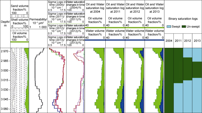
Fig. 4. Illustration of water saturation changes in the reservoir, as identified by cased hole saturation logs and interpreted in “sweep” binary log. |
2.2.2. Generating synthetic saturation logs for each equiprobable model
As spatial fluid property changes are recorded for each individual grid cell, changes of water and oil saturations near the wellbore are also recorded, thus allowing the estimation of synthetic saturation well logs at any time during the simulation period. Synthetic saturation logs can capture the fluid saturation for each grid block located along the path of a specific well.
Information from saturation logs is critical in producers because an increase in water saturation, above a specific threshold, can be related to water breakthrough. Fig. 5 shows an example of a 2D vertical section of water saturation profile along the well trajectory of a pair of producer and injector at a specific point in time during the simulation. Fig. 5 also shows a well log view of the corresponding synthetic water saturation log of the producer well at the same simulation time step.
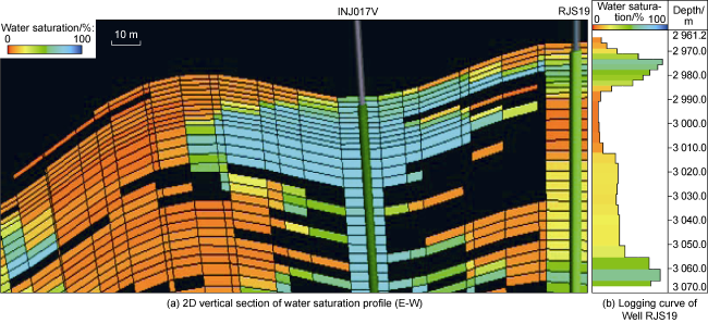
Fig. 5. (a) 2D vertical section of water saturation profile along the well trajectory of a producer and an injector, and (b) the producer synthetic water saturation log. |
As also captured in Fig. 5 , the injected water in the injector well INJ017V has created preferential paths towards the producer RJS19 at the top and the bottom of the reservoir. These preferential waterfront paths are also captured as high-water saturation intervals in the producer synthetic water saturation log.
For the proposed workflow, synthetic saturation logs are generated for all producers with available saturation logs, providing an additional evaluation parameter for validation of the simulation model.
2.2.3. Transforming saturation logs into binary logs using a threshold
To transform the previously generated synthetic saturations logs into binary simulation logs, a water saturation threshold is used. This threshold represents the minimum water saturation of the near-wellbore cells, at the moment the waterfront arrives at the producer well. Classifications in the binary saturation log are obtained as follow: (1) Swept class (after waterfront has arrived). A log segment is classified as swept when the water saturation in specific zones is above the threshold. (2) Un-swept class (dry production). A log segment is classified as un-swept when the water saturation has not yet reached the threshold.
Threshold value of saturation at water breakthrough can be estimated either empirically or analytically, depending on the field data available.
(1) Analytical Method. When special core analysis (SCAL) data is available, the fractional flow curve can be used in combination with the Welge method [16] to estimate the average water saturation at the waterfront. The common procedure to estimate the average water saturation at the waterfront is by drawing a tangent line to the fractional flow curve from the initial water saturation, and the water saturation corresponding to the tangent point is the threshold value. This method relies on the availability of core samples for the different type of rocks and SCAL results from laboratory experiments, and is affected by reservoir characteristics, fluid and reservoir properties and pressure draw-down. The saturation determined from the Welge method is an average saturation and from the mathematical point of view, there are some limitations to determine the exactly tangent point when the fractional curve does not show appreciable changes with water saturation. Results reported by Iscan [17] showed a good match between water saturation values estimated by fractional flow and production logging tools PLT for different rock types.
(2) Empirical Method. As previously captured, water saturation threshold is the near-wellbore water saturation of the producers when water arrives to the well, hence if a saturation log has been recorded at the point of time when a specific well starts producing water, the maximum water saturation in the log can be used as the threshold. This method relies on the availability of water saturation logs at the time the well started producing water.
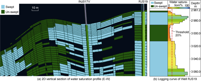
Fig. 6. Swept and un-swept areas of a 2D reservoir model slice highlighting the producer RJS19 and the closest injector at a specific time step. |
2.2.4. Comparing match quality between observed vs synthetic logs by generating a confusion matrix log
Each binary synthetic saturation log, derived from individual models, can be directly compared with the observed binary RST log. The direct comparison process is performed using the confusion matrix classification metrics, after segmenting both observed and synthetic logs in depth units. As a result, a confusion matrix log is created for the entire log depth. Example of Model 1 confusion matrix log and its corresponding confusion matrix table is shown in Fig. 7 .
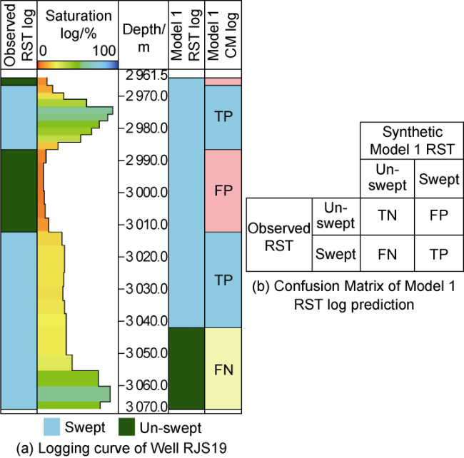
Fig. 7. Confusion matrix log of Model 1 and its corresponding confusion matrix table. |
2.2.5. Assessing history matching quality of individual models using binary confusion matrix derived metrics
During the development of the proposed methodology, the top five widely recommended confusion matrix metrics were assessed to identify the most suitable to address the binary RST mismatch. As result of this assessment, the Matthew Correlation Coefficient (MCC) was selected as the only metric that could numerically represent similarities between observed and synthetic saturation logs. The MCC metric is calculated for all the models in the ensemble. Afterwards, all models are ranked by the MCC metric results, and the best ranked model is selected.
2.3. Geological model used
The UNISIM semisynthetic 3D reservoir model from UNICAMP was used to evaluate the applicability of the new methodology. The chosen geological model was a case study project developed by Cepetro educational centre (UNICAMP University, Brazil). UNISIM is a black oil semi-synthetic sector model built in a high-resolution 3D grid using public data from the Namorado Field, located in Campos Basin (offshore Brazil). One of the main objectives of the development of UNISIM was ensuring that all relevant reservoir geological details were captured to makes UNISIM one of the best benchmarking models to evaluate new methodologies. The Namorado reservoir is located in an anticlinal trap with a bottom driven active aquifer. The field is divided in three main flooding units defined by three depositional sequences separated by discontinuous sequences of marls with poor vertical connection. The reservoir is divided in two main compartments, separated by a sealing fault with two oil-water contacts. The developing strategy of the field considers water injection as pressure support mechanism, with 14 producers, 11 injectors and 7 years of historical production.
A modified high resolution water flooding UNISIM model was used to assess method feasibility and reservoir heterogeneity impact. Modifications introduced to the original UNISIM-I-H model were aimed to increase heterogeneity and waterflooding applicability. Relevant modifications are explained as follow: (1) Model vertical resolution increased. In order to incorporate more heterogeneity to the model, which allows better representation of the reservoir fluid movement, the model grid was subdivided in three separated zones and the vertical cell resolution was increased 2 times in all the zones. (2) Well trajectories. Existing well trajectories were changed from horizontal to vertical to simplify the model for the waterfront monitoring study. In order to expand the model usability and incorporate a more general view of the reservoir development, well trajectories and injection patterns were changed (Fig. 8 ). (3) Porosity and net-to-gross (NTG) log correction. After improving vertical grid resolution and changing the well path to vertical, original porosity and NTG property logs became obsolete. As porosity and NTG logs are inputs required in the stochastic model-built workflow, missing logs were regenerated using data from vertical wells in conjunction with a neural network algorithm. This modification to the model also improves stratigraphic resolution and better vertical NTG can be obtained.
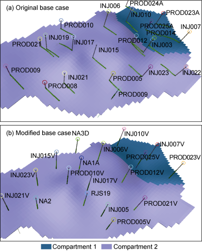
Fig. 8. Injectors and producers well trajectory modification. |
After all model enhancements were done, an uncertainty matrix was created considering the most relevant UNISIM model uncertainties captured by Gaspar [15]. Model modifications and uncertainty ranges defined in the uncertainty analysis were sufficient to generate a diverse initial ensemble of 160 3D models. Fig. 9 shows porosity and permeability diversity of four randomly selected models from one of the ensembles.
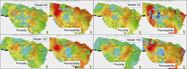
Fig. 9. Porosity and permeability diversity of four randomly selected models from the modified case ensemble. |
After initial ensemble was generated and the base case (case 127) was selected, a final ensemble of 200 models was generated in the second stage of the benchmarking workflow.
To mitigate the uncertainty associated to aggregation methods, one producer observation well and one RST date were identified to be used in the assessment and evaluation of classification metrics. Well RJS19 was selected for this assessment due to its high vertical perme-ability contrast and the date 08/08/2013 was selected as RST date to ensure that the waterfront has already arrived to the well at least in one zone. Additionally, both analytical and empirical threshold calculation were used in this assessment in order to mitigate the uncertainty associated to threshold estimation.
For the empirical method, the water saturation threshold of the observation well RJS19 was estimated using water saturation log and water production data from the base case. For the analytical method, synthetic UNISIM SCAL data was extracted from the base case saturation model and used in combination with Welge method to estimate the threshold.
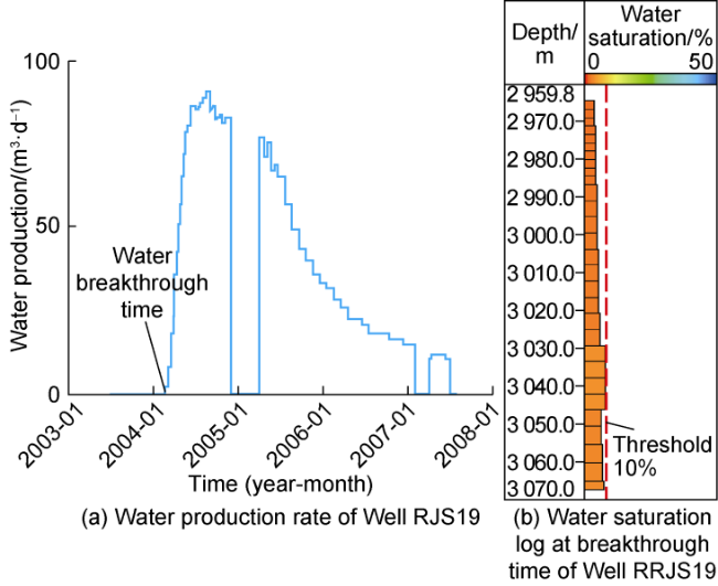
Fig. 10. Empirical threshold estimation using base case water saturation log at the time of water breakthrough. |
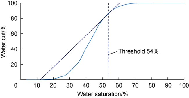
Fig. 11. Water saturation threshold using Welge method. |
3. Method application and discussion
3.1. Assessment and evaluation of classification metrics
This preliminary assessment incorporated the testing and evaluation of the top binary metrics derived from the confusion matrix to quantify the matching quality of saturation logs. As mentioned before, for the binary metric assessment, the observation well RSJ19 was selected to be used as representative well. As a result of this analysis the best binary metric was selected to be used with the proposed methodology.
In order to capture the threshold uncertainty impact into the metric selection, empirical and analytical thresholds estimation methods were used to transform water saturation logs into binary sweep logs for the 200 cases ensemble (defined as Group A and B, respectively). To evaluate the matching quality, individual metrics were used to calculate the RST mismatch and all cases were compared and ranked in each threshold group. After the ranking, the top ten best matching cases were selected from the ranked list to visually compare with the observed RST log for final qualitative analysis of the selected cases.
3.1.1. Precision
For the Group A (empirical threshold), a complete subset of ten cases was selected using precision metrics after the 200 cases were ranked as it is showed in Fig. 12 . However, the expected selection of the top ten best cases was not possible for the group B (analytical threshold) as the first 14 cases shared the maximum precision score as it is showed in Fig. 13 . As has been highlighted by Powers[12] and then corroborated in this analysis, precision metric or True Positive Rate tends to be biased by the positive category, in the RST binary context, the un-swept category.
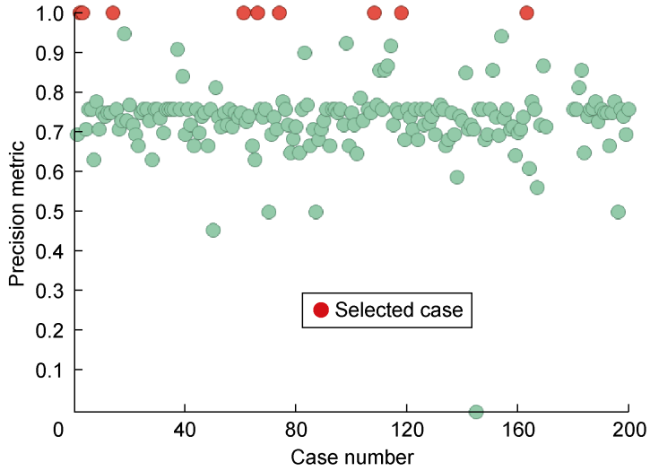
Fig. 12. Precision scores of all 200 models in Group A. |
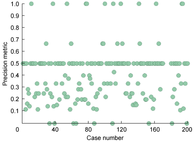
Fig. 13. Precision scores of all 200 models in Group B. |
3.1.2. Accuracy, F-Measure and Recall
Like when using the Precision metric, it was not always possible to select a group of ten cases when using Accuracy, F-Measure or Recall metrics. For some of them a maximum group of six cases was able to be selected. However, it was a norm along these metrics that most of the cases in the ensemble tend to share the same calculated value, which makes impossible to rank the models and select a representative case.
3.1.3. Matthew correlation coefficient
Opposite to the other assessed metrics, a full subset of ten cases were selected using the MCC metric in the group A, and the difference in case scores in the MCC subset allowed the selection of a representative case with the best matching quality (case 37, Fig. 14 ). This metric also allowed the selection of a reduced group of cases if needed. In the Group B, only six cases were able to be selected (Fig. 15 ).
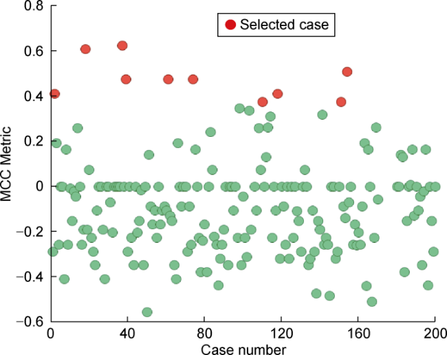
Fig. 14. MCC scores of all 200 models in Group A. |
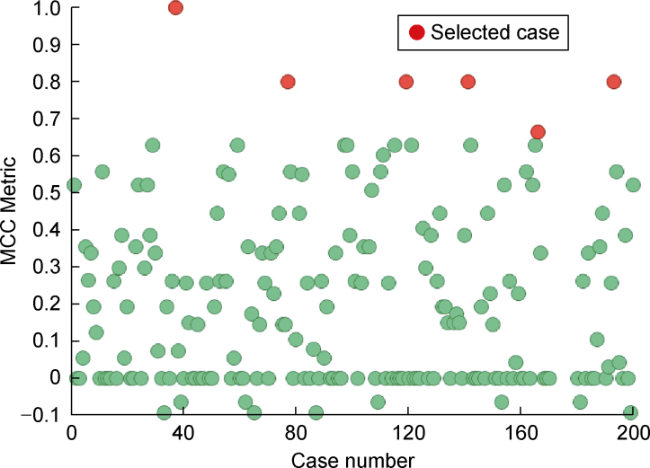
Fig. 15. MCC scores of all 200 models in Group B. |
3.1.4. Binary metrics assessment summary.
A visual comparison of the observed and predicted binary logs for the selected cases using both threshold groups is presented in Fig. 16 . On this figure, dashed yellow lines indicate boundaries between the two categories “swept” and “un-swept”. For the Group A, all the selected cases using the precision metric perfectly match the un-swept category; however, the matching quality of the swept category is inaccurate. Comparable results were observed for the Group B for selected cases using the Recall metric. However, all cases perfectly matched the swept category but show inconsistent results for the un-swept category matching. Unpredicted results were also found for the accuracy and F-measure metrics when comparing both threshold groups. For Group A, both metrics present inaccurate matching for both swept and un-swept categories. For both, empirical and analytical threshold groups, Accuracy, F-measure and MCC metrics selected the same model (37) as top case with best matching quality among the entire ensemble of cases. However, MCC metric is the only metric which selected cases 154 (in Group A), and 166 (in Group B) within the top selected models. Both 154 and 166 cases seem to be visually similar to the observed RST logs, hence they have better history matching quality than other selected cases. MCC metric presented the most balanced results between swept and un-swept classes when compared to observed binary RST, independently of the threshold used.
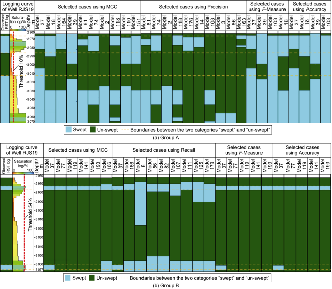
Fig. 16. Evaluation of selected model cases for each metric vs. observed binary RST logs. |
This assessment demonstrated that MCC metric is the best to be used as history matching quality metric when two equally important categories are assessed. Besides, results indicate that the MCC metric can mitigate any category bias by considering all categories equally important to be matched. MCC score distinction adds extra flexibility to the model selection when incorporating additional KPIs into the selection process.
3.2. Comparing proposed RST methodology versus conventional history matching approach
For traditional approach, the selection of the subset of ten cases was performed using a water-cut well based objective function. The objective function was created using standardised RMSE calculation method. For the RST methodology approach, the best ten cases were selected using the MCC metric. For this comparison, data from all producers were included, and for both, conventional and proposed methodologies, global misfits were calculated as cumulative error of individual wells. To facilitate the comparison, global misfits were normalised (0-1). Calculation of the global misfits of the 200 cases and selection of the 10 cases with the best history matching quality was performed for both methods and results are showed in Figs. 17 and 18 . There are two cases which were commonly selected by both methods, the top ranked case (case 37) and case 151 which was ranked differently in both subsets.
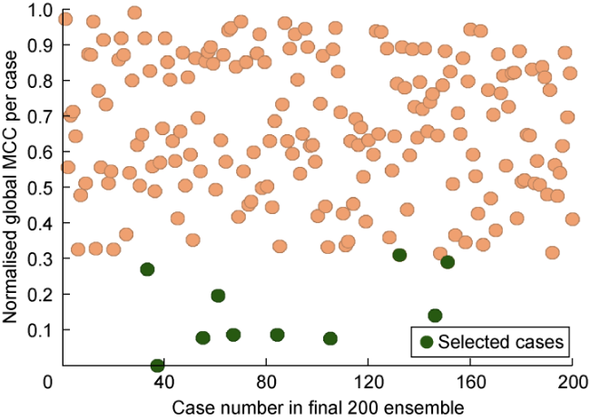
Fig. 17. Global misfits of 200 cases using proposed method. |
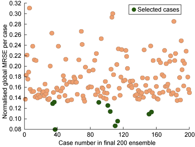
Fig. 18. Global misfits of 200 cases using conventional method. |
Select cases 105 and 110 ranking second in proposed and conventional methods respectively for fitting quality analysis with the base case. For illustration purposes, three representative wells were selected to show history matching quality results of the top ranked cases. Wells NA2, NA3D and PROD021V were selected based on their field location and stratigraphic column in order to capture different heterogeneity degrees of the reservoir properties. Wells NA2 and NA3D have thick and good quality sands, divided by a poor sand interlayer, and PROD021V has poor vertically connected thin sands, separated by small shale layers. Full stratigraphic column of selected wells can be seen in Fig. 19 . As well as the comparison of the base case RST log against RST logs of the two top ranked cases selected from the different methodologies. As expected, near-wellbore saturation of the case selected by using RST methodology (case 105) seems to have a better history matching quality.
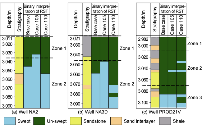
Fig. 19. Binary RST logs of top raked cases for the representative wells. |
Well level water cut results from 3 representative wells are showed in Figs. 20-22. From Well NA2 results, both selected cases seem to have reasonable high-quality match. However, the proposed methodology case seems to outperform the conventional method in wells NA3D and PROD021V.
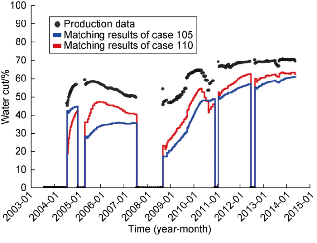
Fig. 20. Well NA2 water cut. |
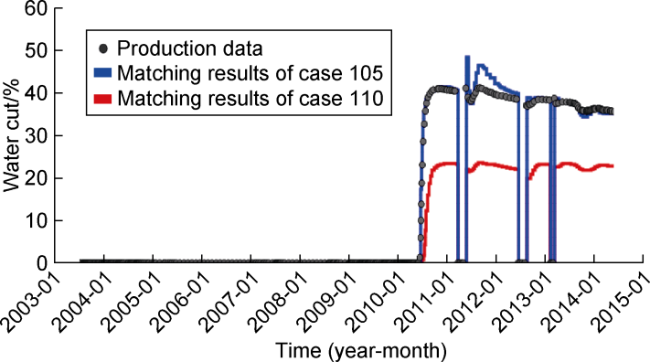
Fig. 21. Well PROD021V water cut. |
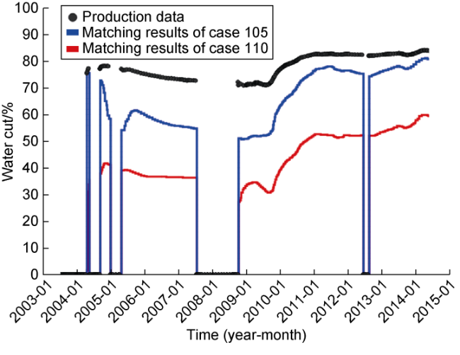
Fig. 22. Well NA3D water cut. |
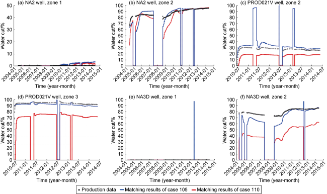
Fig. 23. Water cut per zone for wells NA2, NA3D and PROD021V using conventional and proposed methodologies. |
A global analysis of the obtained results suggests that although the conventional method exceeds on selecting cases where the total water cut of a well is closer to the observed data, it fails to identify the waterfront arrival at different zones as the zonal match is poor. Depending upon model objectives, having a better representation of the actual zonal and intra-zonal water displacement could potentially provide critical information for the decision-making process. For instance, if the purpose of the model is to assess the value of adding or closing well perforations to reduce water production, having a model with detailed representation of the water displacement from different zones is crucial.
4. Conclusions
The proposed methodology has been successfully evaluated using a high-resolution 3D gridding, from public data from the Brazilian Namorado Field model, and saturation logs data to assess the history matching quality in order to understand and select models with better match of sweep pattern. The main conclusions are summarized below:
(1) The history matching quality of a reservoir model can be measured using statistical analysis metrics derived from the confusion matrix, such as the Matthew Correlation Coefficient MCC. MCC metric can mitigate any category bias as it considers all categories as equally important, allowing the selection of more category balanced groups of cases.
(2) The use of binary RST logs as matching parameter improves the selection of models with better history matching quality at zonal/sands level. Reservoir heterogeneity seems to play a significant role when selecting different history matching methodologies. Thus, the use of RST logs as matching parameter contributed the most in highly heterogeneous waterflooded reservoirs.
(3) As expected, the quality of the match when using RST as a matching criteria is highly correlated to the number of RSTs available per well. Approach is less effective when scarce data is available. The history matching quality by well using RST logs for the selected cases relies on the number of RST samples available and the dates when they were taken. Having a better distributed set of RST logs along the history will positively impact selecting a model with better matching quality throughout the entire historical period.
(4) Further studies should be performed when merging both conventional and proposed methodology for history matching processes.