

Introduction
The water injection is the most fundamental and widely used method for oilfield development in China. With the continuous development, major oil fields have generally entered the middle and late stages of development accompanied by rapid decline of production and development efficiency. These oil fields face a series of world-class challenges such as the inadequate demands on effective recovery of remaining oil and technological level [1⇓-3]. There is an urgent need to build a "reservoir-engineering" efficient production system. The refinement management concept needs to be integrated into complete production processes. The real-time monitoring and adjustment of the separated-zone water injection are realized. The combination of real-time production data and static oil reservoir data can be used to deepen geological re-understanding [4]. Liu et al. have broken through important technologies such as under-ground high-pressure permanent flow detection and long-term dynamic sealing [5-6], and developed two technical systems for separated-zone water injection: cable controlled and wave code communicating. They are China's fourth-generation separated-zone water injection technologies and realize digital upgrade to "injecting while measuring and adjusting" in China. Now these technologies have been widely applied. The wave code communicating separated-zone water injection technology does not require to preset cable outside tubing, and can work at pressure. Using injected fluid as a signal carrier, and manual intervention through aboveground or underground control valves, it can provide wireless bidirectional communication, adjust injection rate and obtain production data [7]. This technology has achieved significant results in low permeability to ultra-low permeability reservoirs developed by water injection in Changqing Oilfield.
Many scholars have conducted research on wellbore fluid pulse response models [8]. Through deep analysis on pipeline fluid systems, some foreign scholars understood the mechanism of fluid transport in long-distance suspended pipelines [9-10]. The study results have been applied in deep-sea risers for oil and gas transmission [11]. However, the working conditions in deep-sea risers are very different from separated-zone water injection. Focusing on water injection process, Chinese scholars analyzed the inherent relationship between the pulse transmission parameters of wellbore fluid and wellbore structure and water absorption characteristics of injection intervals [12-13]. In addition, they quantitatively described the pulse response characteristics of data upload and download. However, the research results are almost the interpretation of steady-state pressure and flow measuring points under ideal flow conditions, without considering the effects of fluid viscosity, wellbore structural parameters, and reservoir seepage factors on flow conditions [14]. In addition, there is no description and analysis of the dynamic response process of wellbore fluid, and the response mechanism of pressure and flow states at various points in wellbore is still unclear [15]. For wave code communicating separated-zone water injection, the encoding and decoding of key parameters still rely on engineering experience. It requires conducting research on the dynamic response mechanism of wellbore fluid in water injection wells, which will further improve communication efficiency and provide theoretical basis.
Based on the working conditions of actual separated- zone water injection wells, this paper analyzes the stress and motion state of wellbore fluid microelements, and establishes a pressure-flow rate model for fluid microelements. We extend the microelement model to the whole wellbore flow field, and solve the dynamic spatiotemporal distribution of wellbore fluid flow velocity, pressure, and other parameters by considering the time-domain characteristics of wellbore fluid wave propagation. Then the fluid dynamic response is analyzed, and compared with the traditional Bernoulli equation model without friction loss. Finally, factors such as friction loss, transmission delay, and signal attenuation on the wireless wave code communicating process in water injector are analyzed, which further verifies the accuracy of the model.
1. Dynamic fluid mechanics model
1.1. Pressure-flow rate microelement analysis based on fluid mechanics
The assumption on flow state of the Bernoulli equation for macroscopic hydraulic model is too idealized. It is mainly applicable for static description of ideal states with minimal or negligible fluid viscosity [16], but unsuitable for fluid microelement kinematic analysis, so it cannot meet the requirements of dynamic fine analysis for the whole wellbore. Microelement analysis is a fine method for analyzing fluid mechanics, which has the advantages of clear and intuitive geometric meaning and linear distribution of fluid pressure changes [17]. According to the analysis of actual working conditions of water injection wells, fluid flow in wellbore should meet the following three assumptions: (1) The fluid is laminar flow; (2) The fluid is a Newtonian fluid where the tangential stress at any point in an element is linearly related to the deformation velocity tensor; (3) The fluid element is only subjected to gravity besides stress.
Firstly, based on the spatial position and stress state of a fluid microelement, the resultant stress vector matrix of the fluid microelement is derived. Then, based on the relative motion state between fluid microelements and Newton's internal friction law, fluid viscosity is introduced to obtain the constitutive relationship between stress tensor and deformation velocity tensor. Finally, according to the Newton's laws of mechanics, the relationship between flow velocity field and pressure field of fluid microelements is established.
1.1.1. Stress analysis on fluid microelement
The macroscopic wellbore fluid is gridded into microelements. Establish a three-dimensional Cartesian coordinate system with the direction of wellbore fluid flow as the horizontal axis. The velocity matrix and acceleration matrix of the hexahedron microelement were defined as:
$\begin{matrix} ~u={{\left[ \begin{matrix} {{u}_{x}} & {{u}_{y}} & {{u}_{z}} \\\end{matrix} \right]}^{\text{T}}} \\\end{matrix}$
$a={{\left[ \begin{matrix} {{a}_{x}} & {{a}_{y}} & {{a}_{z}} \\\end{matrix} \right]}^{\text{T}}}$
According to the Newton's second law, the resultant stress matrix of a fluid microelement is:
$\begin{matrix} ~F=ma=\rho dxdydz\left[ \begin{matrix} {{a}_{x}} \\ {{a}_{y}} \\ {{a}_{z}} \\\end{matrix} \right]=\rho dV\left[ \begin{matrix} {d{{u}_{x}}}/{dt}\; \\ {d{{u}_{y}}}/{dt}\; \\ {d{{u}_{z}}}/{dt}\; \\\end{matrix} \right] \\\end{matrix}$
Set the angle between directional fluid element and horizontal direction as α, and the flow is uniform. A fluid element is only affected by gravity and surface forces. Moreover, the pressure matrix applied by an element's own gravity to each surface of the element is:
$\begin{matrix} G=\rho gdV{{\left[ \begin{matrix} sin\alpha & 0 & -\cos \alpha \\\end{matrix} \right]}^{\text{T}}} \\\end{matrix}$
A fluid microelement is subjected to the stresses from adjacent microelements in all directions. Taking the flow direction as the key direction, the stresses applied to a fluid microelement is shown in Fig. 1 where σxb and σxf represent the normal stresses generated by the back and front microelements at the same axis; τxy and τxz represent the tangential stresses generated by deformation in x direction on y and z directions, respectively. The other stress surfaces and the stress states in various directions can be deduced accordingly.
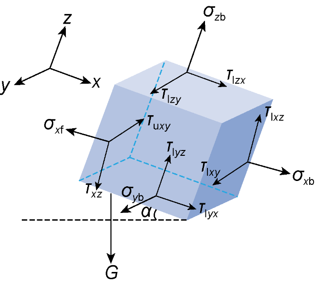
Fig. 1. Schematic diagram of stresses on a fluid microelement. |
Analyzing the composition of the stresses applied on a fluid microelement. Taking the direction in x axis as an example, the directions of the normal stress gradients on both sides of a fluid microelement are opposite, and the expressions for σxf and σxb can be obtained as follows:
$\begin{matrix} {{\sigma }_{xf}}={{\sigma }_{x}}-\frac{\partial {{\sigma }_{x}}dx}{2\partial x} \\\end{matrix}$
${{\sigma }_{xb}}={{\sigma }_{x}}+\frac{\partial {{\sigma }_{x}}dx}{2\partial x}$
Similarly, the normal stresses σyf, σyb, σzf, and σzb acting on the fluid microelement in y and z directions can be derived. Furthermore, the normal stress matrix σp of the fluid microelement is obtained as Eq. (7):
${{\sigma }_{p}}=\left[ \begin{matrix} {{\sigma }_{xb}}-{{\sigma }_{xf}} & 0 & 0 \\ 0 & {{\sigma }_{yb}}-{{\sigma }_{yf}} & 0 \\ 0 & 0 & {{\sigma }_{zb}}-{{\sigma }_{zf}} \\ \end{matrix} \right]=\mathbf{diag}\left( dx\frac{\partial {{\sigma }_{x}}}{\partial x},dy\frac{\partial {{\sigma }_{y}}}{\partial y},dz\frac{\partial {{\sigma }_{z}}}{\partial z} \right)$
The fluid microelement is subjected to tangential stresses from adjacent microelements in the direction along x axis, with opposite stress gradients on both sides. The tangential stresses on top and bottom (τuyz and τlyz) are shown in the Eqs. (8) and (9):
$~\begin{matrix} {{\tau }_{uyz}}={{\tau }_{yz}}-\frac{\partial {{\tau }_{yz}}dy}{2\partial y} \\\end{matrix}$
${{\tau }_{lyz}}={{\tau }_{yz}}+\frac{\partial {{\tau }_{yz}}dy}{2\partial y}$
The tangential stress matrix of the fluid microelement τq is:
${{\tau }_{q}}=\left[ \begin{matrix} 0 & {{\tau }_{lyx}}-{{\tau }_{uyx}} & {{\tau }_{lzx}}-{{\tau }_{uzx}} \\ {{\tau }_{lxy}}-{{\tau }_{uxy}} & 0 & {{\tau }_{lzy}}-{{\tau }_{uzy}} \\ {{\tau }_{lxz}}-{{\tau }_{uxz}} & {{\tau }_{lyz}}-{{\tau }_{uyz}} & 0 \\\end{matrix} \right]=\left[ \begin{matrix} \text{d}x\text{ d}y\text{ d}z \\ \text{d}x\text{ d}y\text{ d}z \\ \text{d}x\text{ d}y\text{ d}z \\\end{matrix} \right]\left[ \begin{matrix} 0 & \frac{\partial {{\tau }_{yx}}}{\partial y} & \frac{\partial {{\tau }_{zx}}}{\partial z} \\ \frac{\partial {{\tau }_{xy}}}{\partial x} & 0 & \frac{\partial {{\tau }_{zy}}}{\partial z} \\ \frac{\partial {{\tau }_{xz}}}{\partial x} & \frac{\partial {{\tau }_{yz}}}{\partial y} & 0 \\ \end{matrix} \right]$
The resultant stress on the fluid microelement is composed of normal stresses and tangential stresses, and its vector matrix eστ is:
${{e}_{\sigma \tau }}={{\sigma }_{p}}+{{\tau }_{q}}=\left[ \begin{matrix} \text{d}x\text{ d}y\text{ d}z \\ \text{d}x\text{ d}y\text{ d}z \\ \text{d}x\text{ d}y\text{ d}z \\\end{matrix} \right]\left[ \begin{matrix} \frac{\partial {{\sigma }_{x}}}{\partial x} & \frac{\partial {{\tau }_{yx}}}{\partial y} & \frac{\partial {{\tau }_{zx}}}{\partial z} \\ \frac{\partial {{\tau }_{xy}}}{\partial x} & \frac{\partial {{\sigma }_{y}}}{\partial y} & \frac{\partial {{\tau }_{zy}}}{\partial z} \\ \frac{\partial {{\tau }_{xz}}}{\partial x} & \frac{\partial {{\tau }_{yz}}}{\partial y} & \frac{\partial {{\sigma }_{z}}}{\partial z} \\\end{matrix} \right]$
According to the Newton’s second law of mechanics, the resultant force F on the fluid microelement can be obtained combing Eqs. (11) and (4):
$\begin{matrix} F={{\left( {{\left[ \begin{matrix} dydz \\ dxdz \\ dxdy \\\end{matrix} \right]}^{\text{T}}}{{e}_{\sigma \tau }} \right)}^{\text{T}}}+G=\left[ \begin{matrix} \frac{\partial {{\sigma }_{x}}}{\partial x}+\frac{\partial {{\tau }_{yx}}}{\partial y}+\frac{\partial {{\tau }_{zx}}}{\partial z}+\rho gsin\alpha \\ \frac{\partial {{\tau }_{xy}}}{\partial x}+\frac{\partial {{\sigma }_{y}}}{\partial y}+\frac{\partial {{\tau }_{zy}}}{\partial z} \\ \frac{\partial {{\tau }_{xz}}}{\partial x}+\frac{\partial {{\tau }_{yz}}}{\partial y}+\frac{\partial {{\sigma }_{z}}}{\partial z}-\rho g\cos \alpha \\\end{matrix} \right]dV \\ \end{matrix}$
1.1.2. Solution to the velocity-pressure relationship of fluid microelements
In the process of wellbore fluid transport, there is a relative motion between fluid microelements, which results in internal friction. To construct the relationship between pressure-flow rate distribution, it is necessary to clarify the constitutive relationship between stress tensor and deformation velocity tensor. According to the Newton's law of internal friction, the constitutive tangential stress matrix eτ of a fluid microelement can be obtained:
$\begin{matrix} {{e}_{\tau }}=\mu \left[ \begin{matrix} 0 & \frac{\partial {{u}_{x}}}{\partial y}+\frac{\partial {{u}_{y}}}{\partial x} & \frac{\partial {{u}_{x}}}{\partial z}+\frac{\partial {{u}_{z}}}{\partial x} \\ \frac{\partial {{u}_{x}}}{\partial y}+\frac{\partial {{u}_{y}}}{\partial x} & 0 & \frac{\partial {{u}_{z}}}{\partial y}+\frac{\partial {{u}_{y}}}{\partial z} \\ \frac{\partial {{u}_{x}}}{\partial z}+\frac{\partial {{u}_{z}}}{\partial x} & \frac{\partial {{u}_{z}}}{\partial y}+\frac{\partial {{u}_{y}}}{\partial z} & 0 \\ \end{matrix} \right] \\ \end{matrix}$
Define eσ and $\overline{{{e}_{\sigma }}}$ as the normal stress matrices of a fluid microelement at dynamic and static states, respectively. The linear relationship between normal stress and normal deformation velocity tensor can be determined according to the Newtonian fluid characteristics. The normal stress on each stress surface of the microelement is the same at static condition (σp), then:
$\left\{ \begin{array}{*{35}{l}} {{e}_{\sigma }}={{a}_{0}}\left( {{e}_{\sigma x}}+{{e}_{\sigma y}}+{{e}_{\sigma z}} \right)I+{{b}_{0}}\mu diag\left( \frac{\partial {{u}_{x}}}{\partial x},\frac{\partial {{u}_{y}}}{\partial y},\frac{\partial {{u}_{z}}}{\partial z} \right) \\ \overline{{{e}_{\sigma }}}=-{{\sigma }_{p}}I \\ \end{array} \right.$
Under static condition, the fluid microelement is not subjected to tangential stresses and the divergence of flow velocity is zero. According to Eq. (14), Eq. (15) can be derived as follows:
$diag\left[ \left( 1-{{a}_{0}} \right){{e}_{\sigma x}}-a\left( {{e}_{\sigma y}}+{{e}_{\sigma z}} \right),\left( 1-{{a}_{0}} \right){{e}_{\sigma y}}- \right.\left. {{a}_{0}}\left( {{e}_{\sigma x}}+{{e}_{\sigma z}} \right),\left( 1-{{a}_{0}} \right){{e}_{\sigma z}}-{{a}_{0}}\left( {{e}_{\sigma x}}+{{e}_{\sigma y}} \right) \right]=0$
Solve Eq. (15) and substitute the result into Eq. (14). The resultant stress on the fluid microelement is composed of normal stresses and tangential stresses. Therefore, by combining Eq. (13), it can be obtained that:
$\begin{align} & {{e}_{\sigma \tau }}={{e}_{\tau }}+{{e}_{\sigma }}=\mu diag\left[ \frac{4\partial {{u}_{x}}}{3\partial x}-\frac{2}{3}\left( \frac{\partial {{u}_{x}}}{\partial y}+\frac{\partial {{u}_{x}}}{\partial z} \right)-\frac{{{\sigma }_{p}}}{\mu }, \right. \\ & \frac{4\partial {{u}_{y}}}{3\partial y}-\frac{2}{3}\left( \frac{\partial {{u}_{y}}}{\partial x}+\frac{\partial {{u}_{y}}}{\partial z} \right)-\frac{{{\sigma }_{p}}}{\mu },\text{ }\frac{4\partial {{u}_{z}}}{3\partial z}-\left. \frac{2}{3}\left( \frac{\partial {{u}_{z}}}{\partial x}+\frac{\partial {{u}_{z}}}{\partial y} \right)-\frac{{{\sigma }_{p}}}{\mu } \right]+{{e}_{\tau }} \\ \end{align}$
Combine Eqs. (16), (3), and (12) to obtain the relationship between the flow velocity field and pressure field of the fluid microelement (Eq. (17)). The results provide a theoretical basis for accurate analysis of wellbore flow field.
$F=\rho dV\frac{\partial u}{\partial t}=dV\left[ \begin{matrix} \mu gra{{d}^{2}}u+\frac{\mu divu}{3\partial x}-\frac{\partial {{\sigma }_{p}}}{\partial x}+\rho gsin\alpha \\ \mu gra{{d}^{2}}u+\frac{\mu divu}{3\partial y}-\frac{\partial {{\sigma }_{p}}}{\partial y} \\ \mu gra{{d}^{2}}u+\frac{\mu divu}{3\partial z}-\frac{\partial {{\sigma }_{p}}}{\partial z}-\rho gcos\alpha \\ \end{matrix} \right]$
1.2. Pressure-flow rate analysis of wellbore flow field
Considering the actual working conditions of water injection, firstly, the three-dimensional fluid microelement velocity-pressure relationship is expressed in a cylindrical coordinate. Additionally, based on the continuity equation of laminar flow, combined with wellbore structure and formation parameters, the pressure distribution and velocity distribution of wellbore flow field are solved.
1.2.1. Spatial flow field analysis based on fluid mechanics
According to flow state analysis, the Reynolds number equation for viscous fluid flow is shown in the Eq. (18). In field, water injection volume is small and flow rate is slow, so the Reynolds number of fluid flow is much smaller than the critical value of turbulence, and the flow can be regarded as laminar flow. The variation in fluid density in laminar flow is minimal and negligible. Therefore, the compressibility of the fluid in wellbore is not considered. It can be concluded that the flow state under water injection conditions meets the following conditions: (1) Due to the pressure pulse amplitude being much smaller than the background pressure, it is a steady flow field in a continuous pipeline; (2) the fluid flow in wellbore is laminar flow; and (3) Neglecting the compressibility of the fluid in the pipe string during production.
$\begin{matrix} Re=\frac{\rho uD}{\mu }=\frac{4\rho {{q}_{\text{v}}}}{\mu \pi D} \\ \end{matrix}$
Due to the mass difference between fluid inflow and outflow within a microelement is the same as the mass change of the microelement per unit time period, the continuity equation for fluid flow is derived:
$\frac{\partial \left( \rho {{u}_{x}} \right)}{\partial x}dV+\frac{\partial \left( \rho {{u}_{y}} \right)}{\partial y}dV+\frac{\partial \left( \rho {{u}_{z}} \right)}{\partial z}dV=\left( \frac{\partial {{u}_{x}}}{\partial x}+\frac{\partial {{u}_{y}}}{\partial y}+\frac{\partial {{u}_{z}}}{\partial z} \right)\rho dV$
The wellbore as a flow channel is a circular convoluted body. To accurately analyze the flow state of fluid in the flow channel under actual working conditions, it is necessary to convert the three-dimensional Cartesian coordinate system into a cylindrical coordinate system (Fig. 2 ). Based on the velocity conversion between Cartesian coordinate system and cylindrical coordinate system, the expressions for the tangential (θ), radial (r), and axial (x) velocity gradients in the cylindrical coordinate system are obtained:
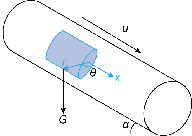
Fig. 2. Fluid microelement velocity in cylindrical coordinate system. |
$gradu=\left[ \begin{matrix} {{u}_{x}} & \frac{\partial {{u}_{r}}}{\partial r} & \frac{r\partial {{u}_{\theta }}}{\partial \theta } \\ \end{matrix} \right]$
Substitute the continuity equation into the velocity-pressure relationship to obtain the expression for the velocity gradient of the fluid microelement when fluid compressibility is ignored:
$gradu={{\left[ \begin{matrix} {{u}_{x}}\frac{\partial }{\partial r}\left( \frac{\partial r}{\partial x} \right) \\ {{u}_{r}}\left[ \frac{\partial }{\partial r}\left( \frac{\partial r}{\partial y} \right)+\frac{\partial }{\partial \theta }\left( \frac{\partial \theta }{\partial y} \right) \right]cos\theta \\ {{u}_{r}}\left[ \frac{\partial }{\partial r}\left( \frac{\partial r}{\partial z} \right)+\frac{\partial }{\partial \theta }\left( \frac{\partial \theta }{\partial z} \right) \right]sin\theta \\ \end{matrix} \right]}^{T}}={{\left[ \begin{matrix} {{u}_{x}}\frac{\partial }{\partial r}\left( \frac{\partial r}{\partial x} \right) \\ {{u}_{r}}\left[ \frac{\partial cos\theta }{\partial r}-\frac{\partial }{\partial \theta }\left( \frac{sin\theta }{\partial y} \right) \right]cos\theta \\ {{u}_{r}}\left[ \frac{\partial sin\theta }{\partial r}+\frac{\partial }{\partial \theta }\left( \frac{cos\theta }{\partial z} \right) \right]sin\theta \\ \end{matrix} \right]}^{T}}$
By combining Eqs. (21) and (20), and substituting into Eq. (17), the pressure-flow rate relationship of fluid microelements in a cylindrical coordinate system can be obtained:
$\left[ \begin{align} & \frac{\partial {{u}_{x}}}{\partial t} \\ & \frac{\partial {{u}_{r}}}{\partial t} \\ & \frac{\partial {{u}_{\theta }}}{\partial t} \\\end{align} \right]=\frac{\mu }{\rho }\left[ \begin{matrix} \frac{{{\partial }^{2}}{{u}_{x}}}{\partial {{r}^{2}}}+\frac{{{\partial }^{2}}{{u}_{x}}}{\partial {{x}^{2}}}+\frac{\partial {{u}_{x}}}{r\partial r}+\frac{{{\partial }^{2}}{{u}_{x}}}{{{r}^{2}}\partial {{\theta }^{2}}}-\frac{{{\sigma }_{p}}}{\mu \partial x}+\frac{\rho gsin\alpha }{\mu } \\ \frac{{{\partial }^{2}}{{u}_{r}}}{\partial {{r}^{2}}}+\frac{{{\partial }^{2}}{{u}_{r}}}{\partial {{x}^{2}}}+\frac{\partial {{u}_{r}}}{r\partial r}+\frac{{{\partial }^{2}}{{u}_{\text{r}}}}{{{r}^{2}}\partial {{\theta }^{2}}}-\frac{2\partial {{u}_{\theta }}}{{{r}^{2}}\partial \theta }-\frac{{{u}_{\text{r}}}}{{{r}^{2}}}-\frac{{{\sigma }_{p}}}{\mu \partial r}-\frac{\rho gcos\alpha }{\mu } \\ \frac{{{\partial }^{2}}{{u}_{\theta }}}{\partial {{r}^{2}}}+\frac{{{\partial }^{2}}{{u}_{\theta }}}{\partial {{x}^{2}}}+\frac{\partial {{u}_{\theta }}}{r\partial r}+\frac{{{\partial }^{2}}{{u}_{\theta }}}{{{r}^{2}}\partial {{\theta }^{2}}}+\frac{2\partial {{u}_{r}}}{{{r}^{2}}\partial \theta }-\frac{{{\sigma }_{p}}}{\mu r\partial \theta } \\ \end{matrix} \right]$
Based on the flow state and the assumption mentioned above, the continuity equation of fluid flow in a cylindrical coordinate system is derived by considering that there are no radial or tangential velocities in the fluid microelement:
$\begin{matrix} ~\frac{\partial {{u}_{r}}}{\partial r}+\frac{{{u}_{r}}}{r}+\frac{\partial {{u}_{x}}}{\partial x}+\frac{\partial {{u}_{\theta }}}{r\partial \theta }=0 \\\end{matrix}$
Substitute Eqs. (21) and (23) into Eq. (22). According to the laminar flow conditions in a circular pipe, the conditions for uniform and stable flow are as follows:
$\left\{ \begin{array}{*{35}{l}} {\partial p}/{\partial r}\;=\rho g\cos \alpha & {} & {} \\ {\partial p}/{\partial \theta }\;=0 & {} & {} \\ \frac{{{\partial }^{2}}{{u}_{x}}}{\partial {{r}^{2}}}+\frac{\partial {{u}_{x}}}{r\partial r}=\frac{\partial p}{\mu \partial x}-\frac{\rho g\text{sin}\alpha }{\mu } & {} & {} \\ \end{array} \right.$
According to Eq. (24), under the continuous flow conditions in a circular pipe, the fluid flow rate and pressure exhibit one-dimensional distribution in the radial and axial directions, respectively. Moreover, by solving the flow velocity distribution, we get the following formula:
$\begin{matrix} ~u=\frac{1}{4\mu }\left( {{r}^{2}}-\frac{{{D}^{2}}}{4} \right)\left[ \frac{\partial \left( p-\rho grcos\alpha \right)}{\partial x}+\rho g\sin \alpha \right] \\\end{matrix}$
In laminar flow, the fluid pressure tends to uniformly decrease in the flow direction. Set the fluid pressure drop per unit length on wellbore as Δpe, the equivalent flow rate is as follows:
$\begin{matrix} ~{{q}_{\text{v}}}=\mathop{\int }_{0}^{2\pi }d\theta \mathop{\int }_{0}^{\frac{D}{2}}urdr=\frac{\pi {{D}^{4}}}{128\mu } \\ \end{matrix}\left( \Delta {{p}_{e}}-\rho gsin\alpha \right)$
The conductivity of continuous pipe flow is Z0=πD4/128μ. In field application, the flow conductivity is related to the roughness of the pipe wall:
$\begin{matrix} ~Z={{k}_{\varepsilon }}{{Z}_{0}} \\\end{matrix}$
The average flow rate in the pipeline is:
$~\begin{matrix} \bar{u}=\frac{4{{q}_{\text{v}}}}{\pi {{D}^{2}}}=\frac{{{D}^{2}}}{32\mu }\left( \Delta {{p}_{e}}-\rho g\sin \alpha \right)=\frac{{{u}_{\max }}}{2} \\\end{matrix}$
1.2.2. Analysis of wellbore flow field
Considering the wellbore structures of water injection wells, the wellbore flow field model is established. For example, a water injection well has measured depth (MD) of l and vertical depth (VD) of h and horizontal angle of α. In the well, there is a micro-section with a length of dl and a VD of dh at lx and hx. The inlet pressure at the micro-section is p1 and the outlet pressure is p2. According to Eq. (26), the flow rate qv in the micro-section can be obtained as:
$\begin{matrix} ~{{q}_{\text{v}}}=\frac{\pi {{D}^{4}}}{128\mu }\left( \frac{{{p}_{1}}-{{p}_{2}}}{\mathrm{d}l}-\rho g\sin \alpha \right) \\ \end{matrix}$
If the trajectory of the whole wellbore is an irregular arc, then the angle between the well section and the horizontal direction is a function of MD and VD, $\varphi \left( {{l}_{x}},{{h}_{x}} \right)$. Set wellhead pressure to be p0, and bottom hole pressure to be ph, and the pressure loss is integrated throughout the whole well section:
${{p}_{0}}-{{p}_{h}}=\mathop{\int }_{0}^{l}\left\{ \frac{128\mu {{q}_{\text{v}}}}{\pi {{D}^{4}}}-\rho gsin\left[ \varphi \left( {{l}_{x}},{{h}_{x}} \right) \right] \right\}dl$
When the well depth tends to infinity, the angle between the tangent direction and the horizontal direction at the inlet is α1, and the angle between the tangent direction and the horizontal direction at the outlet is α2, the spatial structure of the micro-section is shown in Fig. 3 .
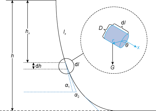
Fig. 3. Schematic diagram of a micro-section. |
The dl is very small, and the corresponding change in deviation angle can be regarded as infinitesimal. Therefore, the micro-section can be regarded as a straight section, that is, the whole well consists of infinite micro-sections with the length of dl. According to the geometric relationship, the following formula can be obtained:
$h=\underset{{{l}_{x}}=0}{\overset{l}{\mathop \sum }}\,\varphi \left( {{l}_{x}},{{h}_{x}} \right)dl=\mathop{\int }_{0}^{l}\sin \left[ \varphi \left( {{l}_{x}},{{h}_{x}} \right) \right]dl$
Combined with the reservoir model, the pressure and flow rate in the whole wellbore are calculated. The bottom hole end communicates with the reservoir, and the bottom hole pressure ph can be regarded as the formation pressure. The water absorption index of the formation is set to be k, and the formation opening pressure is pb. According to the water absorption characteristic model, it can be obtained:
${{p}_{h}}={{k}^{-1}}{{q}_{\text{v}}}+{{p}_{b}}$
Substitute Eq. (29) into Eq. (32). Establish the relationship between wellbore flow rate with wellbore structure, formation characteristic parameters and wellhead pressure, as shown in Eq. (33):
$\begin{matrix} ~{{q}_{\text{v}}}=\frac{\pi {{D}^{4}}k\left( {{p}_{0}}+\rho gh-{{p}_{b}} \right)}{\pi {{D}^{4}}+128\mu kl} \\ \end{matrix}$
When the above equation is combined with Eqs. (25) and (28), the fluid flow velocity distribution in the wellbore can be obtained:
$u=\frac{8k\left( {{p}_{0}}+\rho gh-{{p}_{\text{b}}} \right)}{\pi {{D}^{4}}+128\mu kl}\left( {{r}^{2}}-\frac{{{D}^{2}}}{4} \right)$
According to the pressure gradient distribution for laminar flow, Eqs. (29) and (33) are combined to obtain the pressure px at lx, that is, the spatial distribution of dynamic wellbore pressure:
$\begin{matrix} ~{{p}_{x}}=\left( 1-\frac{128\mu {{l}_{x}}k}{\pi {{D}^{4}}+128\mu kl} \right){{p}_{0}}+ \\\end{matrix}\frac{128\mu {{l}_{x}}k\left( {{p}_{\text{b}}}-\rho gh \right)}{\pi {{D}^{4}}+128\mu kl}+\rho g{{h}_{x}}$
1.3. Time-domain of wellbore fluid wave transmission
The time-domain delayed characteristic of wellbore fluid wave transmission is an important basis for designing wireless communication codec. The fluid wave is generated by the water hammer effect triggered by periodic changes in the opening of throttling elements or changes in pumping pressure (Fig. 4 ). When the flow velocity changes at a point in the wellbore, due to the inertia of the flow section, a shock wave will be induced on the equipment and propagate axially along the wellbore. Set the volume of the flow section to be ΔV, cross-sectional area of the wellbore as A, inside diameter of the pipeline as D, velocity of the fluid wave as c, and thickness of the wellbore wall as e. The fluid section is blocked and compressed by the decrease of the valve opening, resulting in the increase of the total pressure, variation of the fluid density and the flow velocity changing from u0 to u1. According to the momentum principle, the following equation can be obtained:
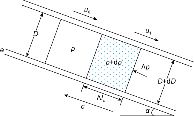
Fig. 4. The generating process of water hammer effect of wellbore fluid wave. |
$\begin{matrix} A\Delta p=\rho gsin\alpha \Delta V-\frac{32\mu u\Delta V}{{{D}^{2}}}+\rho cA\left( {{u}_{0}}-{{u}_{1}} \right)-pA \\ \end{matrix}$
According to the mechanics of materials theory, the physical process of pulse generation is related to tubing material and fluid properties. The fluid elastic modulus E can be calculated according to the relationship between fluid flow continuity and mass conservation (Eq. (37)). The elastic modulus E0 of the tubing is the ratio of the radial stress to the change of the inside diameter after fluid compression. Set the stress variation of the tubing be dσ, and the relationship between the elastic modulus and the strain follows Eq. (38).
$E=V\frac{\text{d}p}{\text{d}V}=\rho \frac{\text{d}p}{\text{d}\rho }$
$\begin{matrix} ~{{E}_{0}}=\frac{\text{d}\sigma }{{\text{d}D}/{D}\;}=\frac{{{D}^{2}}\text{d}p}{2e\text{d}D} \\ \end{matrix}$
Assuming the propagating distance of water hammer wave is Δls (Δls=cΔt) during Δt. The fluid at the far end of the wellbore that has not been subjected to water hammer effect continues flowing into the flow section at its initial rate u0 under the action of inertia, and flows out at u1, resulting in a change in mass within the flow section. Affected by tubing elastic property, the cross-sectional area of the tubing in this flow section increases from A to A+dA, and the fluid density increases from ρ to ρ+dρ. The mass increment of the flow section is:
$\left( \rho +\text{d}\rho \right)\left( A+\text{d}A \right)c\Delta t-\rho Ac\Delta t=\rho A\left( {{u}_{1}}-{{u}_{0}} \right)\Delta t$
The relationship between flow rate, area, and density changes can be obtained:
$\begin{matrix} ~\frac{{{u}_{1}}-{{u}_{0}}}{c}=\frac{\text{d}A}{A}+\frac{\text{d}\rho }{\rho } \\\end{matrix}$
From the relationship between the changes in tubing ID and cross-sectional area, we get:
$\begin{matrix} ~\frac{\text{d}A}{A}=\frac{\text{d}{{D}^{2}}}{{{D}^{2}}}=\frac{2\text{d}D}{D}=\frac{D\text{d}p}{e{{E}_{0}}} \\ \end{matrix}$
After combining Eq. (41) with Eq. (36), we get:
$c=\sqrt{\frac{eE{{E}_{0}}}{\rho \left( e{{E}_{0}}+DE \right)}\left( 1-\frac{1}{2g}\frac{\partial {{u}^{2}}}{\partial {{l}_{x}}} \right)}$
According to laminar flow conditions, the change in fluid flow velocity is minimal compared to the velocity of water hammer wave, but wellbore pressure changes significantly. Therefore, the transmission velocity of water hammer wave is equivalent to:
$c=\sqrt{\frac{eE{{E}_{0}}}{\rho \left( e{{E}_{0}}+DE \right)}}$$\left( \frac{\partial {{u}^{2}}}{2g\partial {{l}_{x}}}\approx 0 \right)$
Some energy of water hammer signals is consumed by tubing friction, resulting in damping attenuation. Set the pressure wave amplitude generated at the throttling element to be Δpl, and the pressure wave amplitude at lx to be Δpx, and the ratio of the two is the attenuation coefficient δx of pulse signal. According to the exponential decay law, it can be obtained:
${{\delta }_{x}}=\frac{\Delta {{p}_{x}}}{\Delta {{p}_{l}}}=\text{exp}\left( -\frac{{{l}_{x}}}{{{l}_{\delta ={{\text{e}}^{-1}}}}} \right)$
where, ${{l}_{\delta ={{\text{e}}^{-1}}}}$is the transmission distance when signal decays to e−1 times its original strength (Δpl), which is related to the signal frequency f. It can be inferred that:
${{l}_{\delta ={{\text{e}}^{-1}}}}=\frac{cD}{2}\sqrt{\frac{\rho }{\pi f\mu }}=D\sqrt{\frac{eE{{E}_{0}}T}{2\pi \mu \left( e{{E}_{0}}+DE \right)}}$
The pulse signal frequency (f) is the switching speed of the throttle element. A single-pulse corresponds to an opening-closing process of the throttling element. The pulse time (T) must be larger than or equal to the transmission delay time (2l/c), and T=1/2f, so we get:
$\begin{matrix} ~f\le \frac{c}{4l} \\ \end{matrix}$
The pressure wave amplitude Δpx at lx after signal attenuation is:
$\begin{matrix} \Delta {{p}_{x}}=\Delta {{p}_{l}}{{\delta }_{x}}=\Delta {{p}_{l}}\text{exp}\left[ -\frac{{{l}_{x}}}{D}\sqrt{\frac{2\pi \mu \left( e{{E}_{0}}+DE \right)}{\rho eE{{E}_{0}}T}} \right] \\ \end{matrix}$
2. Simulation and results analysis
A typical water injection well was selected from an oilfield in China for simulation analysis. The deviated well is with MD of 1600 m and VD of 1400 m. The reservoir opening pressure is 1.5 MPa. The water absorption characteristic index is 25.2 m3/(d•MPa). The working condition is applicable for wave code communicating separated-zone water injection.
2.1. Dynamic distribution of wellbore pressure at constant injection rate
By using the fluid microelement pressure-flow rate model proposed in this paper, and considering the oilfield production performance, we simulated the dynamic distribution of wellbore pressure. The water injection rate for the whole well section is 80 m3/d. The wellhead pressure is 6, 8, 10 MPa, respectively. The dynamic distribution of wellbore pressure along MD and VD directions was simulated and calculated (Fig. 5 ).
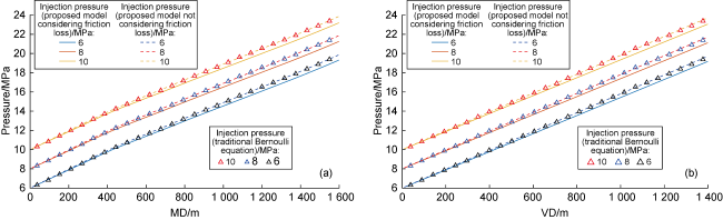
Fig. 5. Dynamic distribution of wellbore pressure along MD (a) and VD (b) directions based on the proposed model and traditional Bernoulli equation. |
The dashed lines in Fig. 5 represent the dynamic distribution of pressure calculated using our proposed fluid pressure-flow rate model without considering friction loss under different injection pressures. The results are consistent with those from the traditional Bernoulli equation, which verifies the accuracy of the proposed model. Therefore, the model can meet the fluid dynamics calculation under the assumed flow conditions (1) to (3) in pressure-flow rate microelement analysis. Moreover, the dynamic distribution of pressure in actual wellbore was calculated, that is, the dynamic simulation considering frictional loss (Fig. 5 ). Affected by friction loss, the wellbore pressure curve moved downward. When the wellhead pressure is 6, 8, 10 MPa, the bottom hole pressure is 19.30, 21.30, 23.30 MPa, respectively (Fig. 5a ), with the difference between the bottom hole pressure at the corresponding dashed line of 0.75 MPa, indicating that the pressure loss along the wellbore is not related to the wellbore pressure. In other words, when designing a wave code communicating encoding and decoding scheme, there is no need to consider the absolute injection pressure, but it should be considered by surface and wellbore equipment and pressure sensors. The wellbore pressure in Fig. 5b exhibits an approximate linear distribution along the VD direction. Additionally, compared with the pressure without considering friction loss, the decrease in bottom hole pressure at different injection pressures is all about 0.75 MPa. The results verify the correctness of the proposed model.
2.2. Dynamic distribution of wellbore pressure at constant injection pressure
Assuming the injection pressure is 8 MPa, injection rate is 60, 80 100 m3/d, respectively, we conducted numerical simulation of the dynamic distribution of wellbore pressure. The simulation results are shown in Fig. 6 . The dashed line represents the dynamic pressure distribution without considering friction loss after stopping water injection. The results are consistent with those of the traditional Bernoulli equation, which verifies the accuracy of our model. The bottom hole pressure at 60, 80, 100 m3/d is 21.72, 21.29, 20.87 MPa, respectively (Fig. 6a ), and differs from the static pressure by 0.18, 0.61, and 1.03 MPa, respectively. The wellbore pressure is approximately linearly distributed along the VD direction (Fig. 6b ). At constant injection pressure, the higher the injection rate, the larger the friction loss along the wellbore is. The model can be used to quantitatively analyze the corresponding relationship between surface pressure and absolute value of bottom hole pressure during wellbore communication.
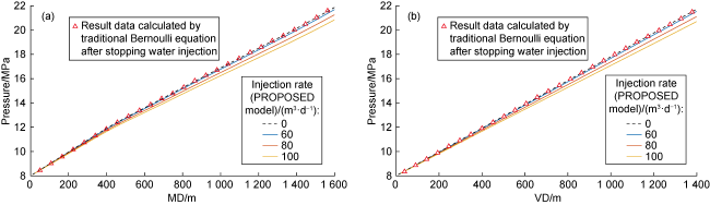
Fig. 6. Dynamic distribution of wellbore pressure along MD direction (a) and VD direction (b) at different water injection rates. |
2.3. Wave code transmission characteristics
Two key parameters for designing a wellbore wave code communication encoding and decoding scheme are signal delay and signal amplitude. Using the water hammer wave velocity model, we studied the delay law of fluid waves in conventional tubing with different sizes to simulate the dynamic response of fluid wave signals (Fig. 7 ). The transmission delay is 1.473, 1.470, 1.462 s at 1000 m, and 2.361, 2.356, 2.343 s at 1600 m, in the three types of tubing with IDs of 50.3, 62.0, 75.9 mm, respectively. The smaller the ID, the longer the delay is. However, the impact is only milliseconds and can be ignored. The delay amplitude mainly depends on the length of the wellbore. In other words, in a longer wellbore, the impact of delay should be considered when designing the encoding and decoding scheme, and the time interval between instruction and data transmission should be longer than the delay time. It is necessary to further study the engineering quantification analysis when considering communication efficiency and bit error rate.
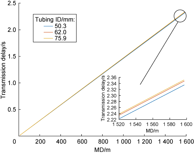
Fig. 7. Delayed characteristic curves of fluid wave signal transmission in three types of tubing. |
By studying the attenuation law of fluid wave signal transmission in tubing with different IDs, we can effectively guide the design of identifiable pressure amplitude in wellbore wave code wireless communication. Pressure with too large amplitude is not detectable. Pressure with too small amplitude may cause excessive loss of hardware resources. The signal attenuation amplitude in tubing with 50.3, 62.0, 75.9 mm ID at 1600 m is 5.50%, 5.05%, and 4.68%, respectively (Fig. 8 ). The smaller the ID, the larger the attenuation amplitude of fluid wave signal is.
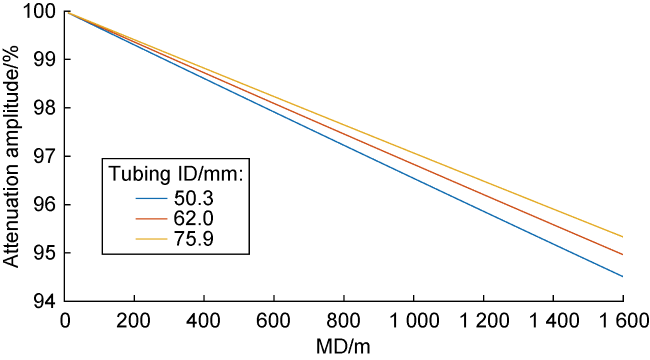
Fig. 8. Attenuation characteristic curves of fluid wave signal transmission in three types of tubing. |
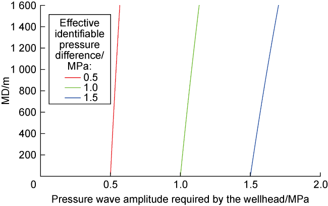
In field application, pressure detection usually has certain errors. It is necessary to analyze the dynamic change of pressure amplitude to realize wireless signal transmission. For the effective pressure difference identified under existing engineering and monitoring conditions, a large pressure difference is more conducive to wireless communication. In the case where the wellhead pressure rises and the pressure difference in low-permeability reservoirs changes little, it is difficult to apply in engineering operation. It is necessary to quantify the pressure change under different working conditions and calculate the effective identifiable pressure difference (i.e., the pressure difference threshold of the sensor) based on formation characteristics to improve communication efficiency. The effective identifiable pressure difference was given in our simulation experiment. At the same time, our model was used to simulate the dynamic distribution of wellbore pressure at different wellhead pressures, and the applicable conditions were quantitatively analyzed (without considering interlayer interference).
The simulation results show that the deeper the well, and the larger the wellhead pressure, the greater the attenuation of the pressure wave signal. When the amplitude of the wellhead pressure wave is 3 MPa, the amplitude of the bottom hole pressure wave is 2.849 MPa, and the attenuation is up to 0.151 MPa. Therefore, it is necessary to improve communication reliability by increasing wellhead pressure change and the accuracy of pressure identification. We simulated the minimum pressure wave amplitude required for the wellhead when the effective values of differential pressure identification at different well depths are 0.5, 1.0, 1.5 MPa, respectively (Fig. 9 ). The area on the right side of the characteristic curve is the range of wellhead pressure wave amplitude values that meet the wireless communication of fluid waves under the constraints of identifiable pressure difference and well depth. The curve characterizes the relationship among effective identifiable bottom hole pressure difference, well depth and the minimum pressure wave amplitude required by the wellhead, which provides theoretical data for the development of effective wellbore wave encoding and decoding scheme at different well depth conditions.
Fig. 9. Characteristic curves of effective identifiable pressure difference and pressure wave amplitude required by the wellhead. |
3. Conclusions
Based on the microelement analysis method for fluid mechanics, we establish a fluid microelement pressure-flow rate model and extend it to the whole wellbore flow field. Moreover, based on the time-domain characteristics of fluid wave propagation in the wellbore, a dynamic spatiotemporal distribution model of flow rate and pressure in the wellbore is obtained. Based on the production data of a typical water injection well, we conduct numerical simulation and find that the pressure loss along the wellbore is independent of the absolute injection pressure. Therefore, when designing a wave code communication encoding and decoding scheme, it is not necessary to consider the absolute injection pressure. When the injection pressure is constant, the higher the injection rate, the larger the friction loss along the wellbore is. The delay of fluid wave signals depends on the length of the wellbore. The smaller the tubing ID, the larger the attenuation of fluid wave signals is. The higher the amplitude of the target wave code generated at the same well depth (the effective identifiable pressure difference), the greater the amplitude of the wellhead pressure required to overcome the friction loss along the wellbore. The model can provide a mechanism model and theoretical data for optimizing the efficiency of wave code communication in separated-zone water injection.
Nomenclature
a—acceleration of fluid microelement motion, m/s2;
a—acceleration matrix of a hexahedron microelement, m/s2;
a0—coefficient of normal stress term on fluid microelement, dimensionless;
b0—coefficient of constitutive relationship term for fluid microelement, dimensionless;
A—cross-sectional area of tubing, m2;
c—fluid wave propagation velocity, m/s;
D—tubing ID, m;
e—thickness of tubing wall, m;
eσ—normal stress matrix of a moving fluid microelement, Pa;
$\overline{{{e}_{\sigma }}}$—normal stress matrix of a static fluid microelement, Pa;
eτ—constitutive tangential stress matrix of a fluid microelement, Pa;
eστ—resultant stress on a fluid microelement, Pa;
E—elastic modulus of fluid, Pa;
E0—elastic modulus of tubing, Pa;
f—fluid wave frequency, Hz;
F—resultant force on a fluid microelement, N;
g—gravitational acceleration, m/s2;
G—gravity matrix of a fluid microelement, N;
h—vertical depth of a whole well, m;
hx—vertical depth at a point in a wellbore, m;
I—unit matrix;
k—formation water absorption index, m3/(s•Pa);
kε—material coefficient, dimensionless;
l—measured depth of a whole well, m;
lx—measured depth at a point in a wellbore, m;
Δls—length of the flow section with water hammer effect, m;
m—microelement mass, kg;
p—fluid pressure, Pa;
pb—formation opening pressure, Pa;
ph—bottom hole pressure, Pa;
px—pressure at lx from the wellhead, Pa;
p0—wellhead pressure, Pa;
p1—inlet pressure of the micro-section, Pa;
p2—outlet pressure of the micro-section, Pa;
qv—volume flow rate, m3/s;
Δp—pressure difference, Pa;
Δpe—fluid pressure drop per unit length of wellbore, Pa/m;
Δpx—pressure wave amplitude at lx, Pa;
Δpl—pressure amplitude at the throttling element, Pa;
r—radial distance in a cylindrical coordinate system, m;
Re—Reynolds number, dimensionless;
t—time, s;
Δt—time interval, s;
T—period of pulse signal, s;
u—fluid rate, m/s;
u—fluid rate matrix of a hexahedron microelement, m/s;
$\bar{u}$—average flow rate, m/s;
u0, u1—flow rate before and after fluid compression, m/s;
V—fluid volume, m3;
ΔV—volume of the flow section, m3;
x, y, z—Cartesian coordinate system, m;
Z—practical conductivity coefficient, m4/(s•Pa);
Z0—conductivity coefficient of continuous tubing, m4/(s•Pa);
α—angle between fluid microelement and horizontal direction, (°);
α1—angle between the tangent line at the inlet of the well section and the horizontal line, (°);
α2—angle between the tangent line at the outlet of the well section and the horizontal direction, (°);
δx—signal attenuation coefficient, dimensionless;
θ—polar angle in cylindrical coordinate system, (°);
μ—fluid viscosity, Pa•s;
ρ—fluid density, kg/m3;
σ—normal stress on a fluid microelement, Pa;
σp—normal stress matrix on a fluid microelement, Pa;
σp—normal stress on the stress surface of a static fluid microelement, Pa;
σxb, σyb, σzb—normal stresses perpendicular to the stress surface of the microelement generated by the back microelement at x, y, z axis, Pa;
σxf, σyf, σzf—normal stresses perpendicular to the stress surface of the microelement generated by the front microelement at x, y, z axis, Pa;
τ—tangential stress on a fluid microelement, Pa;
τq—tangential stress matrix on a fluid microelement, Pa;
τxy, τxz—tangential stresses generated by deformation in x direction on y and z directions, Pa;
τyx, τyz—tangential stresses generated by deformation in y direction on x and z directions, Pa;
τzx, τzy—tangential stresses generated by deformation in z direction on x and y directions, Pa;
ϕ—angle between a well section and the horizontal line, which is a function of well MD and VD, (°).
Subscripts:
u, l—top and bottom surfaces of a microelement perpendicular to the axis;
max—maximum value.