

Introduction
Drilling in an oil and gas field is an inevitable step for extracting natural resources. As it is a cost-intensive process, the wells must be drilled at limited and calculated locations to improve the predefined objective function of the field development plan (FDP). However, each well perforates only a few square feet of the total formation. With a limited number of wells, one can extract information from only a few square kilometers. Thus, reservoir is largely unknown as the ratio of the volume of drilled area to the entire reservoir is negligible. It is thus vital to work with uncertainty to make the best decisions for the FDP.
Incorporating uncertainty allows the operators to embrace the situation more competently and mitigate the risk of failure. It is common to extract new information through field evaluation. Assimilating such information is helpful to update the uncertainty quantification and further improve decision-making under uncertainties. However, obtaining new information during the appraisal phase also comes at an exorbitant cost. Therefore, most decisions relevant to the FDP (number, locations, and type of wells, operational settings, and other decision variables) are made using the information before drilling the first development well. Consequently, this process yields a sub-optimal FDP [1]. With this in mind, numerous workflows have been developed to revise FDP under uncertainty and improve the objective function of the project. Closed-loop field development (CLFD) [1⇓⇓⇓-5] is one such workflow. CLFD is a feedback-based field development process that uses data on newly drilled wells and their production over time. Such new wells and their well-testing results, among other sources of information, provide new insights into the fluid flow and reservoir characteristics. CLFD systematically accrues and assimilates such information in multiple phases to update reservoir scenarios. Finally, these scenarios are used to optimize the objective function by revising the FDPs.
Loomba et al. [1] identified several limitations in prior studies on CLFD. They highlighted the presence of negative or ambiguous results reported in previous studies [2⇓⇓⇓-6,16]. These findings raise concerns about the applicability of existing workflows in practice. Moreover, the use of simple 2D or 3D models by Shirangi et al. [2], Kim et al. [5] and Hanea et al.[16] further questions their practicality and ability to address the complexities of actual field development. Hidalgo et al. [4] failed to demonstrate significant differences in well locations between the optimized FDPs of cycle 0 and cycle 1, despite conducting over 1000 experiments. The authors also overlooked the negative bias resulting from the strong correlation between the decreasing number of wells and increasing monetary gains. Similarly, Hanea et al. [16] focused only on optimizing the drilling sequence in a simple 3D example, neglecting the challenges associated with field development and still obtaining negative outcomes in one of their examples.
Efficiency is another area where all previous studies fall short. All existing workflows are very time-consuming and unrealistic for practical applications. Although Loomba et al. [1] validated their workflow on two 3D case-studies, their workflow is very inefficient. The authors generated 500 petrophysical images to perform data assimilation before selecting representative models (RMs), with 1600 scenarios per RM during the optimization process. But, unlike theoretical studies, even a single reservoir model of an actual oil and gas field can consume long hours for simulation [7⇓-9]. It is thus infeasible to simulate tens of thousands of full physics-based simulations using the CLFD workflow of Loomba et al. [10]. Another critical aspect often overlooked in prior studies is the total time required for a CLFD cycle. While previous authors assumed CLFD as an instantaneous process, in reality, decision-making can take weeks to months.
By consolidating these shortcomings identified in the previous research, our study aims to present an improved and efficient CLFD workflow. The incorporation of these insights enhances the validity and practicality of our proposed approach, leading to more accurate and informed decision-making processes in field development. We work on an extensively time-consuming model as theoretical 3D studies do not capture the time-consuming nature of actual oil and gas reservoir models. Thus, we strive to overcome the limitations of previous workflows by working with realistic examples that entail long hours of simulation under uncertainty. A machine learning (ML) assisted optimization process is also presented in this work to predict the behavior of the partially simulated scenarios, which is used to demonstrate that partial simulations can be used to predict the field’s behavior and drastically reduce computational time.
1. Objectives
While the general objective of this work is to recurrently revise FDP under uncertainty, the specific objectives are listed below:
(1) Present an efficient CLFD workflow for practical applications. As a CLFD workflow consists of multiple steps, it is important to strike a balance to ensure that uncertainty quantification and assessment are done effectively.
(2) Validate the workflow on a giant benchmark field, with extensively time-consuming physics-based simulation models. As most studies only use simple synthetic models, it is essential to validate the workflow on a time-consuming and field-scale example to understand its utility.
(3) Optimize net present value (NPV) of the field as the objective function of the FDP using limited decision variables in a quarter of the giant field.
(4) Introduce an ML-assisted technique to accelerate optimization process. Unlike conventional methods, intermediate results obtained by running simulations over partial life are used to optimize the project’s objective function. The newly proposed cluster-based learning and evolution optimizer (CLEO) [11] algorithm is used to explore the problem space intelligently for such complex applications.
(5) Introduce a routine for working with multiple approved scenarios to maximize the likelihood of success and expedite the CLFD workflow. The concepts of propagation of best experiments and increasing representative models (RMs) with iterations are introduced. The probability of success of the selected FDP in each cycle of CLFD is presented.
(6) Establish the benefit of a CLFD workflow by including its execution time and working with realistic timelines.
(7) Revise the FDP without any uncertainty reduction. In other words, data assimilation using only historical production and well-logs are the only components providing a new understanding about the reservoir. Such rigorous conditions provide an excellent setup to understand the benefit of data assimilation (DA) process in a CLFD workflow.
(8) Discuss the key observations, potential pitfalls of CLFD workflow and provide necessary recommendations for practical applications.
2. Methodology
Loomba et al. [1] introduced a comprehensive and validated CLFD workflow. The workflow requires a large ensemble of reservoir simulation models to work with field’s uncertainty. They used 500 petrophysical images to assure a reliable coverage of geological uncertainty during field development. However, using as many as 500 scenarios can be impractical for real applications, as presented by several authors [7⇓⇓-10]. These facts raise two riveting questions regarding: (1) how to determine the number of scenarios for the success of CLFD, and (2) how to revise FDP for real applications that are extensively time-consuming.
Ideally, a CLFD workflow must be as efficient as possible, as it serves to improve prior decisions during the highly uncertain development phase. Bearing this in mind, we present an efficient and risk-informed workflow to make CLFD workflow viable for real applications. This CLFD workflow includes the steps below (Fig. 1 ):
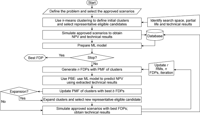
Fig. 1. Flowchart of the algorithm to optimize FDP. |
(1) Action. Generate petrophysical realizations to capture the geological uncertainties during this phase of acquiring first-hand information.
(2) Update inputs. Prepare the initial ensemble of scenarios combining updated uncertainty attributes along with geologically consistent petrophysical images.
(3) Data assimilation. Assimilate the noisy production data and minimize its mismatch with the simulated ensemble.
(4) Approved scenarios. Carefully examine the ensemble of posterior scenarios to discard the unlikely scenarios to mitigate their negative impact on the decision- making process.
(5) Select RMs and optimize. Efficiently optimize using the concepts of ML, propagation of best experiments (PBE) and growing RMs with iterations. The process uses CLEO as the core optimization algorithm. We discuss the critical elements of this alogrithm below:
(1) ML model: The main purpose of using an ML model is to exponentially improve the efficiency of the optimization process. An ML model is a program trained with a dataset using a learning algorithm (for example, linear regression, logistic regression, decision tree, random forest algorithm). A trained ML model can perceive patterns and predict the behavior of a previously unseen dataset. In this work, we used random forest regression as the learning algorithm. In random forest regression, a collection of decision trees is created, each trained on a different subset of the data. Each decision tree independently predicts the target variable based on a set of input features. The final prediction is then obtained by averaging or taking the majority vote of the predictions from all the individual trees. The strength of random forest regression lies in its ability to handle complex relationships between the input features and the target variable, as well as to handle high-dimensional datasets. It is also robust to outliers and noise in the data.
In this work, the CMG software is applied to simulate the approved scenarios and obtain their NPV to prepare the dataset. We extracted technical results from the simulated approved scenarios at different time steps. Such technical results involve scalar parameters such as cumulative oil produced, gas-oil ratio, and water-oil ratio, and grid parameters such as net flux oil, net gas, and net water. We also calculate the parameters for grids near the well (see Reference [10] for details). Structuring this labeled data together, we train the ML model. During each iteration, simulate the reservoir scenarios over a limited life of the field rather than the complete lifecycle. We extracted the technical results for this period and prepared them for the ML model. The trained ML model predicts the NPV for the lifecycle of the field. Then the best FDP in the iteration was used to simulate the approved scenarios again for the complete lifecycle and extract the labeled dataset. Finally, we updated the ML model using this dataset before moving on to the next iteration.
(2) Propagation of best experiment (PBE). To limit the number of simulations, Loomba et al. [10] introduced the idea of PBE, which selects the best FDPs over a gradually incrementing subset of RMs within an iteration of the optimization process. Only these selected FDPs are tested with the next subset of RMs. The process is repeated until all RMs have been considered (see Reference [10] for details). The main objectives of using PBE are reducing the total simulations and improving the likelihood of success of the optimized FDP over the ensemble.
(3) Increasing RMs with iterations. We also integrate the concept of growing RMs with iteration [10,12] in conjunction with the risk-averse objective function presented by Loomba et al. [6]. While the former reduces the number of simulations, the latter is a risk-averse approach to maximize the chances of success in the real field.
(4) Cluster-based learning and evolution optimizer (CLEO). In this work, we used CLEO as the core optimization algorithm. CLEO is a user-friendly optimization algorithm that deftly deals with extensive decision variables and problem space. See Reference [11] for details about this algorithm.
The workflow was built on the fundamentals of Loomba et al. [1], but their workflow lacks features to make it practical for real field applications. We revised the proposed workflow on a giant-field benchmark case, and compared it with the workflow of Loomba et al. to clarify the differences.
3. Application and results
3.1. Benchmark case
In this work, UNISIM-III, a giant-field benchmark case study was used. This synthetic reservoir was created to study and applied on Brazilian pre-salt fields [13-14]. The giant field consists of karsts and volcanic rocks, within a carbonate-depositional environment. The benchmark case study includes an ensemble of simulation models (UNISIM-III-2022) to capture uncertainty; and a reference case (UNISIM-III-R) which emulates the “true field”. For a detailed explanation of the simulation and reference models, we refer the readers to Reference [14].
This giant field is divided into four sectors (Fig. 2a ), with the sectors sequentially developed. The sectors communicate with each other and each one corresponds to a production platform. For sustainable development, 100% of the gas produced is re-injected into the reservoir. The authors also found that applying water-alternating gas maximizes oil recovery. Fig. 2a shows an FDP in UNISIM-III-2022 with 33 producers and 32 injectors scattered across the field. 14 of these wells (Fig. 2b ) were drilled within the first 1219 d of field development.
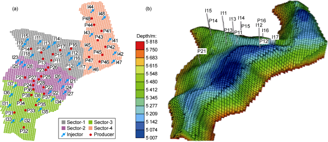
Fig. 2. (a) Sectors distribution and (b) grid-map of UNISIM-III-2022 (the first and second numbers in the well’s nomenclature refer to the sector and drilling sequence, respectively). |
In this work, we only focus on optimizing the field’s net present value (NPV) using the decision variables from Sector-2 (S2): (1) Thirteen out of seventeen development wells of Sector-1 are already operational before the first cycle of CLFD. (2) Despite working with limited decision variables from only a quarter of the field (i.e., S2), the full-field models were adopted to include the impact of neighboring sectors for making a well-informed decision [10]. One must note that the locations of the wells of other sectors are considered fixed for all three cycles. Only to-be-drilled wells of S2 are revised using the accrued information over time. (3) Although the decision variables of S2 were optimized, we assimilated newly acquired information (well-logs, production data, etc.) from all four sectors. (4) Since our study target is the entire field, taking one or all sectors employing CLFD has little difference in execution time. (5) Sector-2 is with the maximum influence from neighboring sectors (Fig. 2a ). Thus, it is a good sector for testing our predictive analytics-based optimization process.
Loomba et al. [11] assimilated data in 1219 d to optimize the NPV of the “true field” by 13%, using undrilled wells (of all four sectors) as the decision variables. We used their optimized FDP as our initial strategy. Table 1 chronologically summarizes the major activities in the field with additional information on the execution of each cycle of CLFD. We considered a period of 3 months to drill, complete, and produce for each well. Only one well per sector is drilled at a given time. At 1219th day, Cycle 0 (pre-CLFD) was executed; at 1978th day, Cycle 1 was executed to revise the blocks of 7 to-be-drilled wells in S2; at 2404th day, Cycle 2 was executed to revise the location of 4 to-be-drilled wells in S2 and finally, at 3531th day, Cycle 3 was executed to revise the blocks of 4 to-be-drilled wells in S2.
Table 1. Summary of relevant activities and information for UNISIM-Ⅲ-2022 |
| Period/d | Drilling, completion and production activity | Remarks |
|---|---|---|
| 0-1219 | 6 producers (P11-P16) and 7 injectors (I11-I17) in S1; producer P21 in S2 | Extended well test performed in S1 in the first year followed an idle 1.4 years |
| 1308-2039 | 4 producers (P22-P25) and 4 injectors (I21-I24) in S2; 2 producers and 2 injectors in both S3 and S4 | |
| 2039-2315 | 1 producer (P26) and 2 injectors (I25, I26) in S2; 2 producers and 2 injectors in both S3 and S4 | |
| 2404-2769 | 2 producers and 2 injectors in both S3 and S4 | |
| 2769-3134 | 2 producers and 2 injectors in S1 | All wells drilled in S1 |
| 3592-3957 | 2 producers and 2 injectors in S2, S3, and S4 each | All wells drilled in S2, S3, and S4 |
| 4322 | ~39% contractual life | |
| 5053 | ~46% contractual life | |
| 11 019 | Field abandonment |
3.2. Cycle 1 of CLFD
The first cycle of CLFD uses the production information of 0-1978 d. By using the ensemble-smoother with multiple data assimilation (ES-MDA) [15], we limited our work to 100 scenarios. The steps are provided below: (1) Generate 100 images of porosity, permeability and rock-types using 27 well-logs (including 13 new logs from wells drilled after 1219 d); (2) Using noisy production data over 5.4 years (1978 d), the data assimilation is performed for 100 scenarios, combining uncertainty attributes and geostatistical images; (3) Approve scenarios from the posterior ensemble of scenarios (only 44 were approved in this cycle); (4) Use the proposed workflow to efficiently revise the FDP with the accrued information; (5) Execute the optimization process using multiple RMs over ten iterations to improve all 44 simulation scenarios by a median value of 2.3%.
By implementing the optimized strategy in the reference case, we improved the NPV by 0.8%. Major improvement in oil recovery factor comes from S3 (1.0 percentage points) and S2 (0.5 percentage points). A larger change in recovery factor of S3 demonstrates how the revised decision in S2 helped the neighboring sector. Meanwhile, it stresses the importance of working with the entire field rather than isolated models when making a holistic decision for the complete field. The percentage change in oil recovery (at the end of Cycle 1) for individual wells is shown in Fig. 3 . A similar trend between expected and actual percentage change in cumulative production is observed, with some exceptions (P45, P16, P42, P47 and P25). Such differences may occur because of various factors, including the uncertainty attributes, like faults close to such wells. It is intriguing to observe how even limited changes made in S2 can affect the wells in S4 (several kilometers away).
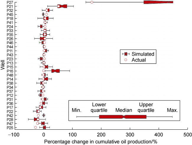
Fig. 3. Percentage change in cumulative oil production of respective wells at the end of Cycle 1 (to make the graph legible, we truncated the result of P27 as the maximum change was observed as high as 1500%). |
It is also vital to maximize the likelihood of success and measure it with the number of improved scenarios, especially when working with a huge uncertainty. In Cycle 1, we improved all the scenarios. To supplement this observation, we also calculated the probability of success of the selected FDP using Z-transformation (a kind of mathematical transformation of a discrete series) of the percentage change in results for each RM. The probability of success (or percentage change greater than 0) of the selected FDP in the true field was observed to be 99.5% in Cycle 1.
The efficiency of this cycle was benchmarked against the first cycle of Loomba et al. [1] (Table 2 ). It can be seen that the efficiency of method in this work has improved by 89%.
3.3. Cycle 3 of CLFD
Like Cycle 1, we implemented CLFD workflow on subsequent cycles 2 and 3. In Cycle 3, the field had been developed for 9.7 years (3531 d), as about 32% of the field’s life. Unlike previous cycles, we assumed that fault transmissibility uncertainty is reduced by Cycle 3. We therefore used a range of 0 to 0.5 for faults transmissibility across the field (rather than 0 to 1).
However, we came across a critical problem in Cycle 3, which resembles practical concerns in the real field development. An extremely high gas-oil ratio (GOR) was observed in producer P17 (well from S1). As the well had been active for a considerable time, we did not consider this observation as an outlier. Given that P17 is drilled in proximity to S2, it is vital to ensure that our models depict this behavior. However, the simulated GOR of P17 was much lower than this observed GOR (Fig. 4 ) even after assimilating production data with ES-MDA. Assuming good connectivity between injectors and P17 as a solution to this problem, we proposed a channel connecting producer P17 and injector I17 to find a workable solution (Fig. 5a ). In Fig. 5b , one can observe that the gap between the simulated and actual GORs of P17 is narrowed greatly after revising data assimilation.
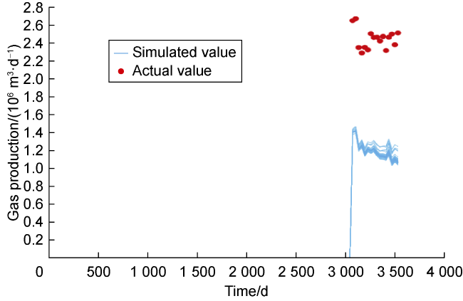
Fig. 4. Gas production of P17 after the initial data assimilation process. |
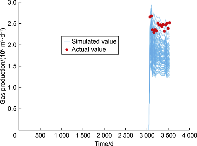
Fig. 5. Gas production of P17 after revising data assimilation. |
Poorly history-matched models constrained us to repeat the data assimilation process in Cycle 3, leading to extra time. To accommodate these necessary changes, time spent on the data assimilation process was commensurate to the optimization process. As such, Cycle 3 took the longest time among the three cycles. In Fig. 6 , one can also observe the corresponding changes. Well P27, placed in proximity to the unbeknownst channel in Cycle 2, was moved further away by the end of Cycle 3.
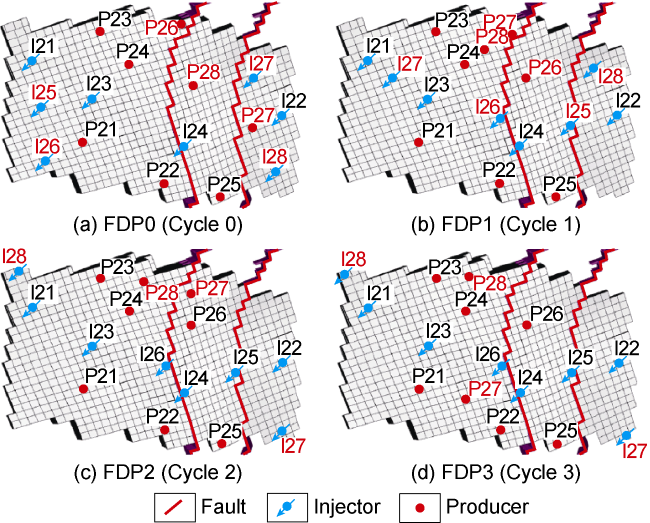
Fig. 6. Best FDP obtained at the end of each cycle (to-be-drilled wells are highlighted in red). |
3.4. Outcome
Table 3. Details of our workflow in all CLFD cycles |
| Cycle | Implementation of workflow | Probability of success/% | Execution time/d | Range of EVoCL/ USD 108 | EVoCL (for ensemble of AS)/USD 108 | VoCL/USD 108 | ||||
|---|---|---|---|---|---|---|---|---|---|---|
| Action | Update input | Data assimilation | Approved scenarios (AS) | Optimization | ||||||
| 1 | Obtained 0+7+3+3 new well logs (from S1, S2, S3 and S4, respectively); Generated Mprior,1 using a total of 27 vertical well-logs | Noisy production data over a period of 1978 d (18% of the field’s life) was used to obtain Mpost,1 | 44 | FDP0 was optimized to obtain FDP1. We used 26 (59% of the AS) scenarios to optimize using 10 iterations of CLEO. Complete ensemble was improved. | 99.5 | 32 | 0.3-5.0 | 2.5 | 0.8 | |
| 2 | Obtained 0+4+5+5 new well logs (from S1, S2, S3, and S4, respectively); Generated Mprior,2 using a total of 41 vertical well-logs | Noisy production data over a period of 2404 d (22% of the field’s life) was used to obtain Mpost,2 | 48 | FDP1 was optimized to obtain FDP2. We used 30 (62.5% of the AS) scenarios to optimize using 7 iterations of CLEO. 94% of the ensemble was improved. | 91.3 | 27 | -0.4-1.8 | 0.7 | 1.1 | |
| 3 | Obtained 4+0+4+4 new well logs (from S1, S2, S3, and S4, respectively); Generated Mprior,3 using a total of 53 vertical well-logs | Range of fault transmissibility was modified from 0-1 to 0- 0.5 for all four faults | Noisy production data over a period of 3531 d (32% of the field’s life) was used to obtain Mpost,3 | 40 | FDP2 was optimized to obtain FDP3. We used 24 (60% of the AS) scenarios to optimize using 7 iterations of CLEO. 90% of the ensemble was improved. | 88.1 | 34 | -0.3-1.6 | 0.5 | 0.8 |
Working with only limited decision variables from a quarter of this giant field, we were able to improve the field’s NPV by USD 2.7×10⁸ (increase rate 2.5%) which emphasizes the merits of implementing an efficient CLFD workflow. Fig. 7 shows the evolving NPV over cycles. Very high uncertainty in the models can be observed at the initial phase of field development. The degree of uncertainty is decreased with the evolving ensemble during development. Growing optimism in the evolving ensemble implied by a sharply increasing median NPV is obtained compared to the true field’s NPV. Assimilating newly accrued information over multiple phases of field development can be beneficial to decrease uncertainty and improve predictive capability.
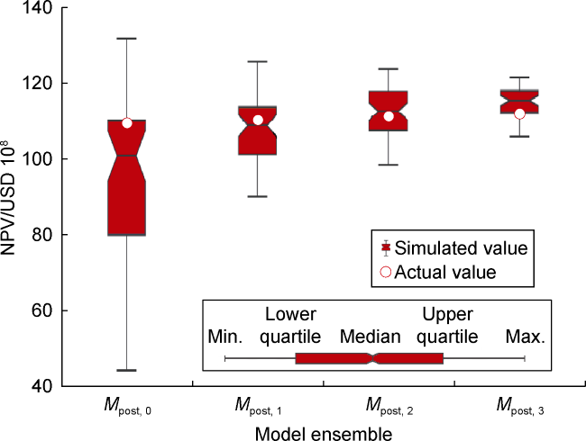
Fig. 7. Simulated and actual NPVs for all cycles. |
Table 4. Predicted recovery factor at the end of all cycles |
| Cycle | Recovery factor/% | ||||
|---|---|---|---|---|---|
| S1 | S2 | S3 | S4 | Entire field | |
| 0 | 36.3 | 31.4 | 36.0 | 29.3 | 33.1 |
| 1 | 36.3 | 31.6 | 36.3 | 29.3 | 33.2 |
| 2 | 37.1 | 31.7 | 36.3 | 29.6 | 33.5 |
| 3 | 36.9 | 33.0 | 36.3 | 29.2 | 33.7 |
4. Discussion and recommendations
This work focuses on revising the FDP using the CLFD workflow, specifically addressing efficiency and risk-informedness. Unlike previous studies that only tested their workflows on simple and fast synthetic models, the method of this work considers the time-consuming nature of reservoir models in actual fields. Table 5 highlights the key differences between our work and that of Loomba et al. [1], underscoring the importance of efficiency in CLFD.
Table 5. Key differences between Loomba et al. [1] and this work |
| Step | Loomba et al. [1] | This work | Remarks |
|---|---|---|---|
| Action | Generated 500 images | Generated 100 images | 80% reduction in time |
| Update inputs | Generated 500 scenarios with updated inputs | Generated 100 scenarios with updated inputs | 80% reduction in time |
| Update inputs | Generated 500 scenarios with updated inputs | Generated 100 scenarios with updated inputs | 80% reduction in time |
| Approved scenarios | ~50% scenarios approved | ~45% scenarios approved | A larger ensemble of approved scenarios is only justified if RMs can be selected without any simulation |
| Select RMs | Selected 9 RMs; only these RMs were used for optimization | Selected 3-12 RMs per iteration; different subset of RMs per iteration | Varying RMs helps reduce time and include more scenarios to make better decisions |
| Optimize | IDLHC was used to optimize well-place- ment using 1600 experiments per RM | Combined ML model with CLEO algorithm | Over 90% reduction in time |
4.1. Efficiency improvement and risk control
In a CLFD workflow, results propagate from one step to another. One must be mindful of the quality of these results to avoid failure of the complete workflow [6]. Hence, we presented a holistic solution to make the efficiency of the workflow improved by 85%. Using this efficient workflow, we recurrently revised the FDP of an extensively time-consuming model in about 30 d, a much acceptable timeframe.
The quality of being risk-informed is equally critical in a CLFD workflow. Adding to the discussion of Loomba et al. [1], we present new insights for practical implementation of a risk-informed CLFD workflow:
(1) Action. The depositional sequence plays a dominant role in the recovery process. Hence, one should construct the ensemble of geostatistical images using multiple geologically consistent scenarios. Considering efficiency, the number of geostatistical realizations generated and used for subsequent steps is another concern. Loomba et al. [1] used 500 realizations in their work, asserting that a large ensemble is necessary to capture the geological uncertainty. However, using as many as 500 realizations to develop a time-consuming model can be impractical. As such, this work uses only an ensemble of 100 realizations to work with time-consuming models. Despite using an 80% smaller ensemble on a highly heterogeneous and giant field fraught with various complexities, the revised workflow worked. This fact raises the question regarding the apt size of the ensemble for a successful understanding of geological uncertainty.
(2) Update inputs. In this work, we revised the FDP without including any direct information (i.e. known and identified information, without any uncertainty) [1] to test the workflow in a challenging environment. Regardless, this step is key to reducing uncertainty during the field's development phase. One should estimate the impact of all unknown uncertainties which can be used to make an informed decision for subsequent steps. For example, one should focus to approve the scenarios that include more impactful uncertainty attributes. Such a risk-informed step bolsters the likelihood of success of the outcome, particularly when one improves all scenarios.
(3) Data assimilation. Several processing activities are involved to separate the extracted liquids. While the total hydrocarbon extracted from the field is measured more accurately after such processes, the well production data is bound to suffer with higher noise. Also, depending on the availability of gauges, only limited well parameters (for example, total liquid rate and bottomhole pressure) may be available to perform data assimilation. It is therefore important to include more subjective knowledge of the field to improve the data assimilation process under such complications. In practice, the true reservoir characteristic of an oil and gas field is unknown. But using a benchmark case gives us the advantage of studying the "true answer" after executing all cycles of CLFD. We capitalized on this fact and revised the DA process in Cycle 3. Re-evaluating the uncertainty parameters, we realized that fractures running along the fault were the primary reason for the observed discrepancy. This observation highlights three aspects. First, unknown uncertainty attributes can cause mismatched production data. Second, as the reference case was built independently of the simulation model, it is common to encounter differences. Such differences helped us demonstrate problems from real situations. Third, such fractures only distributed in proximity of the fault. However, as the scale of the reference and simulation models is quite different, simulation models are not able to capture this behavior of fractures, even after DA. With the large differences in the scale, it is quite unrealistic to portray this behavior accurately as the DA cannot identify such instances. We can affirm this further based on the results obtained using channel to simulate the faults. In summary, a better DA technique is also required to work with a much larger noise and, without any huge uncertainty attributes. To improve DA in such problematic instances, we could also use local grid refinement in addition to new uncertainty parameterization to understand the mismatched area better.
(4) Approving scenarios to select and optimize RMs. In this work, we used reservoir engineering insights alongside the CLEO algorithm. One of its benefits in the CLFD workflow is that it helps prevent drilling a well in an unproductive region by using the data of the approved scenarios. This also helps mitigate the need for correctional steps, like flexibility of drilling (FoD) [1]. Meanwhile, to improve reservoir engineering insights, we need better ways to include the impact of different factors, like faults. For example, if there is a sealing fault close to the well, we need better techniques to incorporate this information and use zero oil flux from that direction. We also need to maximize the likelihood of success over the approved scenarios to ensure success in the "true field". Maximizing the expected monetary value (EMV) of the RMs alone does not ensure its success in the "true field". One must maximize the percentage improvement in the EMV as well as the scenarios improved. Using a growing set of RMs in conjunction with a risk-averse objective function is a good way to efficiently reach that objective. At the same time, a higher probability of success in the true field does not assure a lower mismatch between the expected and actual value of CL. There are perceived similarities between the concepts of (1) growing RMs with iteration and (2) propagation of best experiment (PBE). For example, both of them can improve efficiency of the optimization process, work with multiple realizations. And for a given subproblem, the total number of realizations is fixed. Nonetheless, they have some dissimilarities. The former solves a series of subproblems with increasing RMs, while the latter works with only one optimization subproblem. For growing RMs with iteration, the number of realizations is increased as we advance from one subproblem to the next; while for PBE, the number of realizations is increased within one subproblem only. The former was designed to handle as many realizations as possible, irrespective of how many of them are actually being improved, while PBE was developed to obtain a solution which improves all realizations within the subproblem. The former runs all simulations within a subproblem; thus, it does not improve efficiency within a subproblem. In contrast, PBE runs only a selected simulation; thus, it improves efficiency within a subproblem. The former has a high overall efficiency as it controls all subproblems, while the efficiency of PBE (as a standalone) is comparatively lower as it only acts a supplementary tool within a subproblem. In short, both frameworks supplement rather than substitute each other. As Loomba et al. [11] highlighted, we can achieve a globally optimal solution with simulation models. But, as model error always exists, the solution may be far from a globally optimum solution when applied in a real case. As such, we suggest using predictive analytics to make the optimization process faster. For a better prediction model, we could also use a more detailed feature matrix and effective learning algorithms. Learning feature importance to pick the best features for the feature matrix is another important step to improve the prediction model.
4.2. Considerations in practical implementation
Depending on the size of the field, number of processors, average simulation time per model, and other computational capabilities, it can take weeks to months to revise the FDP. Nevertheless, we must ensure that FDPs can be revised within a realistic time frame. For a practical implementation of the workflow, it is also vital to include decision-making time as delays in oil production can directly impact the NPV and, at times, render the changes in FDP useless. As none of the previous works considered this decision-making period, we included it to exhibit the practicality of our workflow. While roughly 30 d were required by all the cycles for revising FDP, we added an extra 30 d to include the unforeseen managerial and engineering decisions. This extra buffer period also explains the benefit of CLFD workflow in case of additional unexpected delays.
The execution time of the workflow also raises the concern of it being a continuous process. Assuming it takes 30 days to simulate the whole CLFD workflow, the only additional information at this point, in most of the cases, would be a single noisy production data per well. As this additional information may not be value-additive, CLFD requires deliberate planning to maximize its value.
In addition, the number and size of cycles are two independent variables of CLFD. All authors have highlighted the benefit of increasing the number of cycles in CLFD. However, the number of cycles should be increased cautiously to avoid the disadvantageous in certain cases. For example, in the presented example, no new well logs are acquired between 1219-1756 d. In other words, no new spatial and temporal information is acquired for the to-be-developed sectors 2, 3 and 4, so ill-informed decisions may be taken, which can arbitrarily lead to success or failure. On the other hand, cycle size depends on the quantity of information it puts forward. So, for a successful implementation of CLFD (with adequate size and number of cycles), it is recommended to carefully recognize the amount of information, time consumed by CLFD workflow, objective function, and time of executing the workflow, among other things.
4.3. Results of implementation
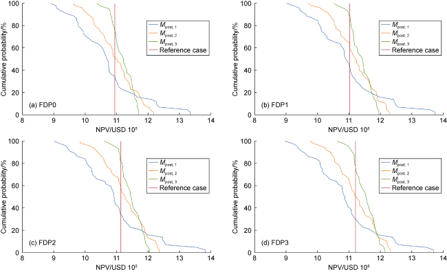
Updated ensemble of each cycle demonstrated similar characteristics (Fig. 8 ):
Fig. 8. Results of revised FDP in Mpost,1, Mpost,2, Mpost,3 and reference case. |
(1) Reduction in volatility. Decreasing coefficient of variation highlights the lower dispersion. For a given FDP, the sharply decreasing standard deviation can be observed in evolving data-assimilated ensemble.
(2) New information reduces uncertainty. Increasing minimum and decreasing maximum values led to a continually decreasing range of NPVs. Unrealistically optimistic and pessimistic values were ruled out from subsequent ensembles.
(3) Growing optimism. For a given FDP, the median NPV is always less than true value in the initial ensemble and ending up over the true value in the final ensemble, as shown in Fig. 8 . This observation suggests that the ensembles are evolving to become more optimistic.
(4) Improved forecast. Despite growing optimism and large uncertainty reduction, the actual value of the field always falls within the prediction results of simulated models. This improves the predictive capability of evolving ensembles. At the same time, this does not necessarily imply that an individual cycle would always induce a positive change as it depends on the percentage of scenarios improved, among other things.
In this work, we only use a few wells (within a sector) as decision variables to optimize the objective function (NPV) of the entire field. Thus, it is understandable that the improvements are not significant as the decision variables in other sectors that play a critical role in the field behavior are not altered. In S2, however, the improvement of NPV is large, which exposes the benefit of CLFD in improving the field’s NPV. This setup also helps indicate the benefits of the ML-assisted CLFD workflow more clearly. The results also demonstrate the benefit of new information coming in the form of noisy production data. Even without updating new inputs in the simulation model during the earlier cycles, an ample change can also be observed.
Additionally, we mitigated bias related to the optimization process by starting with the initial strategy (that is, the optimized strategy proposed by Loomba et al. [11]) before executing Cycle 1. Given the great uncertainty and dearth of information, this FDP is not good enough for updated reservoir scenarios. At the same time, the optimized FDPs from the later cycles are also not amongst the best FDPs for the initial ensembles. These observations highlight two things: (1) the initial strategy is adequate for the uncertainty at the initial stage of field development, and (2) lack of information in the early phase of development misleads to suboptimal decisions.
With the implementation of each cycle, the new information is expected to reduce uncertainty with moderate degree rather than drastic change. For practical implementation of a CLFD workflow, we recommend using performance indices to ensure model variability. Descriptive statistics and image processing can be used to measure the variability at each phase of the cycle and maintain diversity in models. This step is essential to embrace key insights and differences from multiple scenarios. Maximizing the likelihood of success over such a variable ensemble would guide the geoscientists and engineers to select a more robust FDP.
5. Conclusions
By addressing the research gaps in closed-loop field development (CLFD), we present an efficient and risk-informed workflow that enables robust decision-making. Unlike previous studies, we applied the workflow to a highly heterogeneous and giant field with time-consuming simulation models, and validate the functionality of the CLFD workflow in complex conditions characterized by spatial and temporal complexities. A ML model is integrated for predicting objective functions, thereby expediting the workflow. A routine for working with multiple approved scenarios is defined and implemented, and the concept of propagating best experiments is introduced. The cluster-based learning and evolution optimizer (CLEO) is used as the core algorithm in CLFD applications. The use of probability of success is introduced to assist decision-making based on the results observed in the approved ensemble. In addition, we addressed the inclusion of realistic timelines and emphasized the importance of considering the total time for executing a cycle of CLFD to mitigate associated biases. It is confirmed that successful quantification and assessment of uncertainty can be achieved using an ensemble of as low as 100 scenarios.
A significant improvement in NPV is achieved, further highlighting the practical applicability of our approach. The effectiveness of the proposed workflow has increased over 85% in realistic scenarios, validating its functionality in complex reservoir conditions.
Furthermore, we discussed the challenges and considerations in the data assimilation process. A practical problem related to data assimilation due to a non-mapped uncertainty attribute has been demonstrated and resolved, highlighting the necessity of risk-informedness. While the evolving ensemble improves forecasts with reduced volatility, it is important to remain cautious of the growing optimism in the models. To maximize the likelihood of success and generate robust outcomes, we provided practical recommendations, including the utilization of risk-averse objective functions, the generation of diverse scenarios, performing sensitivity analysis on uncertainty attributes, and leveraging information sources like time-lapse seismic.
Acknowledgments
This work was conducted with the support of Libra Consortium (Petrobras, Shell Brasil, Total Energies, CNOOC, CNPC) and PPSA. The authors are grateful for the support of the Center for Energy and Petroleum Studies (CEPETRO-UNICAMP/Brazil), the Department of Energy (DE-FEM-UNICAMP/Brazil), and the Research Group in Reservoir Simulation and Management (UNISIM-UNICAMP/Brazil). Also, a special thanks to CMG and Schlumberger for the software licenses. The authors would also like to acknowledge the contribution of Vinícius de Souza Rios (Equinor/Brazil).
Nomenclature
b—number of best FDPs available;
Mprior,1, Mprior,2, Mprior,3—ensemble of models before data assimilation in cycles 1, 2 and 3, respectively;
Mpost,0, Mpost,1, Mpost,2, Mpost,3—ensemble of models after data assimilation in cycles 0, 1, 2 and 3, respectively;
n—number of FDPs;
r—number of RMs.