

Introduction
The use of horizontal wells is now an important procedure in the petroleum industry. Although the production of horizontal wellbore is larger than that of vertical wellbore, the cost of horizontal drilling is expensive compared to vertical drilling. The increase in production in the horizontal wellbore is affected by many factors such as the flow patterns that occurred due to the difference in the flow rate of multiphase inside the horizontal wellbore, which induce pressure drop in the wellbore and thereby affect the production. Doan et al. [1] indicated that the casing perforation affects the oil production because it causes pressure drop. Marett et al. [2] investigated the friction through perforations by using Darcy law and friction flow that occurs in the horizontal wellbore. It was elaborated that the production was affected by friction pressure drop, which occurred along the perforated horizontal wellbore. The friction may cause an increase in the fluid that enters through the downstream region. However, the fluid flow may be reduced by passing it from downstream to the upstream region at the end of the horizontal wellbore and perhaps induce the reverse flow. Brekke et al. [3⇓⇓⇓⇓⇓⇓-10] illustrated that when incrementing the density of the perforations, the friction factor increased too. It has been observed that the friction factor was increased with the turbulent flow and drag effect. Olson et al. [11⇓⇓-14] investigated the relation between friction pressure drop and flow through perforations (radial flow) in a perforated horizontal pipe, and illustrated that the friction pressure drop increases with the roughness or perforation density. Arshad et al. [15] utilized pipes with different diameters to study the pressure drop and production through the horizontal wellbore. It was observed that the pressure drop was almost constant along the wellbore through the large-diameter pipe, and this can be attributed to the low flow velocity inside the wellbore. Moreover, it was noted that the friction factor was found to be insignificant in production when different diameters of pipes were used. Novy [16] remarked that an increase in the diameter of the wellbore might reduce the friction and hence increase the production. Liu et al. [17-18] studied the production in horizontal wells and observed found that the production depended on the thickness of the reservoir and wellbore pressure. They applied a new method to the four adjusting wells in the Bohai B oil field, and the errors were little enough to be used in determining the production in the offshore oil field. King et al. [19⇓⇓⇓⇓⇓⇓⇓-27] investigated productivity through the horizontal wellbore, and observed that the production was dependent on the length of the wellbore, reservoir anisotropy and perforation density. The production was found to increase with the increasing of these parameters. Tang et al. [28] and Du et al. [29] studied the production and flow efficiency through horizontal wellbores using slotted-lines or perforations, and they observed that the perforation depth and perforation phase angle have a lower influence on the pressure than perforation density, and the effect of the slotted-line was less important compared to the perforations. Moreover, the production increased when the density of the perforations near the heel region (perforations at the outlet section) of the horizontal wellbore increased. Dankwa et al. [30] investigated the production through the horizontal and vertical wellbores. It was observed that the production increased with the wellbore length in the horizontal wellbore while vertical productivity is unaffected by the wellbore length. The production was increased by increasing the thickness of the reservoir through the horizontal and vertical wellbore.
The study of the effect of perforation density on oil production before was only based on a single setting where the increase in perforation density was only made at the wellbore outlet section. Furthermore, only a single-phase condition was considered. In this work, a numerical model for simulating two-phase flow in a horizontal well is established under two perforation density distribution conditions (i.e. increasing the perforation density at inlet and outlet sections respectively). The simulation results are compared with experimental results to verify the reliability of the numerical simulation method. Then, the behaviours of the total pressure drop, superficial velocity of air-water two-phase flow, void fraction, liquid film thickness, air production and liquid production that occur with various flow patterns are investigated under two perforation density distribution conditions based on the numerical model.
1. Laboratory experiment
The experimental apparatus for simulating the two- phase flow in the horizontal wellbore is illustrated in Fig. 1. The main pipe was made of Perspex (acrylic pipe) with a length of 3 m and an internal diameter of 0.038 1 m. The horizontal pipe was designed with 24 perforations (diameter of 0.004 m), opened vertically on the pipe with a phasing angle as 180°. Two perforation density distribution conditions were designed, i.e. increasing the perforation density at inlet and outlet sections, respectively. The perforation spacing is 15 cm and 30 cm in the sections with and without increased perforation density, respectively. Under the two perforation density distribution conditions, nine experimental cases were respectively designed (1n-9n, and 1d-9d, where “n” denotes the condition of increasing the perforation density at the outlet section, and “d” denotes the condition of increasing the perforation density at the inlet section), with the water flow rate set at 35 L/min and the air flow rate at 0.05, 0.10, 0.30, 0.50, 1.00, 3.00, 5.00, 10.00 and 15.00 L/min. The transparent pipe was used to facilitate photography of the flow patterns that resulting from the difference in the superficial velocities of air and water. A high-speed camera (Vision Datum LEO720S) was used, with a resolution of 720×540 pixels and a recording range used at 100-1 000 fps. A centrifugal pump was used to inject axial water flow into the main pipe. An electro-air compressor was used to inject radial air flow through the perforations. The change of flow pattern in the wellbore was observed, and the static pressure drop in the wellbore was measured.
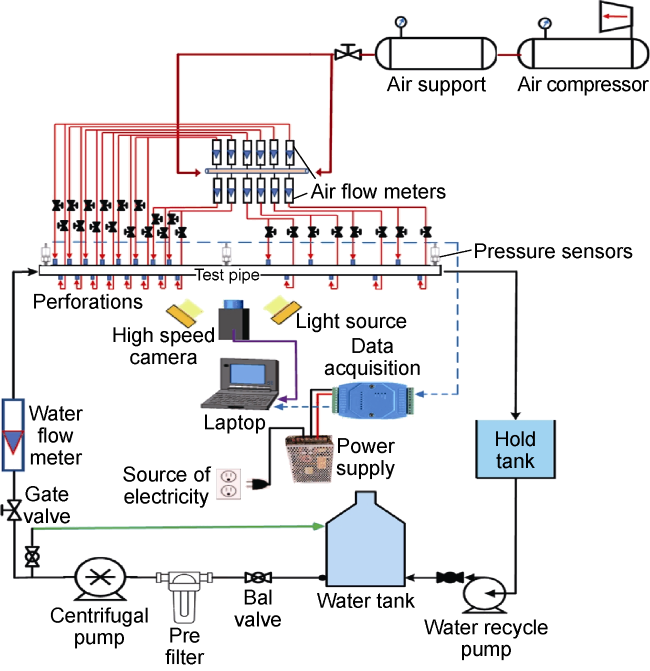
Fig. 1. Experimental setup. |
2. Numerical model
A commercial CFD software, ANSYS Fluent, was utilized to predict the two-phase flow inside the perforated horizontal wellbore, with the same parameters as the laboratory experiment. The 3D computational domain was created within the ANSYS R3 geometric creation module with tetrahedron-type mesh used to resolve the flow field. The computational domain of the perforated horizontal wellbore is illustrated in Fig. 2 , where water and air flow along the x and y directions respectively. A half-symmetry horizontal pipe along the y-direction is developed to optimize the computational time required to solve the sets of governing equations. The symmetric boundary condition was set to constrain the flow pattern, velocity mixture profile, total pressure drop, void fraction and liquid film thickness inside the perforated horizontal wellbore, so that the computational time required to complete the whole calculation can be reduced, without compromising the accuracy of the final solution.
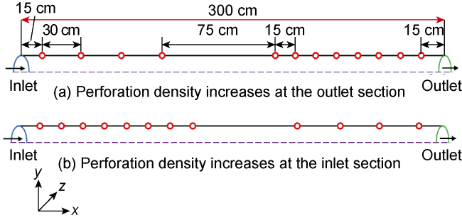
Fig. 2. Computational domain of the perforated horizontal wellbore. |
The grid dependency study was carried out by taking two different sizes of mesh, 70 000 cells (coarse mesh) and 1 100 000 cells (fine mesh), with five inflation layers to solve the viscosity in the turbulent flow that occurs with layers near the wall of the pipe, as shown in Fig. 3. Grid independence has been demonstrated through the perforated horizontal wellbore depending on the regular shape of the bubble flow pattern, and the time taken to achieve convergence has been reduced.
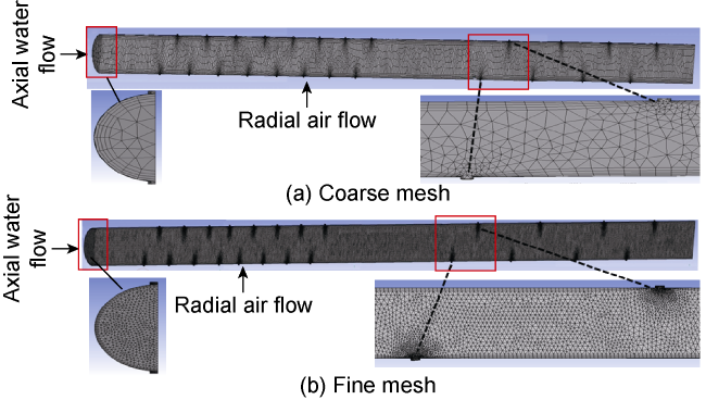
Fig. 3. Computational domain with different meshes. |
The ANSYS Fluent program was used with the volume of fluid (VOF) model that analyses the homogenous model to simulate the two-phase flow patterns in the perforated horizontal pipe. The pressure-implicit with splitting of operators (PISO) method was adopted to solve the pressure-velocity coupling equation. The pressure staggering option (PRESTO) method was utilized with the second-order upwind scheme to solve the momentum equation and pressure interpolation. The renormalization group (RNG) and differential viscosity models were used to simulate the turbulent flow and adjust the mesh density near the wall. In this study, the air phase was considered as the first phase, while the second phase was the water phase; assuming the volume fraction of water was 1 to the wellbore, which means the wellbore was filled with water, and then air entered to get a more accurate distribution pattern. Considering the influence of contact angle on the composition of the bubbles, the contact angle for air phase with water phase was set at 36°, being compatible with the interface [31-32]. The ratio of time step to mesh element size was set as 1×10⁻³, 1×10⁻⁴, 1×10⁻⁵ s/m depending on the complete flow patterns in the perforated horizontal wellbore and also the convergence of the simulation. The simulation took approximately 10 d when the coarse mesh was used, with 9.4 s per iteration, and more than 15 d when the fine mesh was used, with approximately 13.6 s per iteration. The simulation time was further increased when there was a transition between flow patterns, i.e., the transition from bubble to stratified flow and from stratified wave flow to annular flow. This was due to the fact that the fluctuation intensified with an increase in the air flow rate when the water flow rate was constant. The void fraction of flow patterns under coarse and fine meshes was determined when the air flow rate is 0.10 L/min and the water flow rate is 35 L/min by configuring bubble flow. As illustrated in Fig. 4 , the fine mesh yields better results than the coarse mesh, with clearer boundary for the flow patterns. It was observed during the use of the coarse mesh that the bubble flow was unclear due to the impact of the interface (region of film thickness) that separated the bubbles. The void fraction of the air phase was closer to a stratified flow pattern because the bubbles generated will not be separated through the exit from the top perforations. The bubble flow pattern is more apparent with the fine mesh due to the impact of the surface tension and the shear stress. In this study, fine mesh was used with 1 100 000 cells. Based on the experimental scheme mentioned above, simulation cases (1n-9n, and 1d-9d) were designed, with the same flow rates as in the experiment.
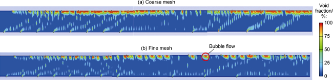
Fig. 4. Distribution of void fraction in horizontal wellbore with different mesh densities. |
3. Model verification
3.1. The behavior of flow patterns in perforated horizontal wellbore
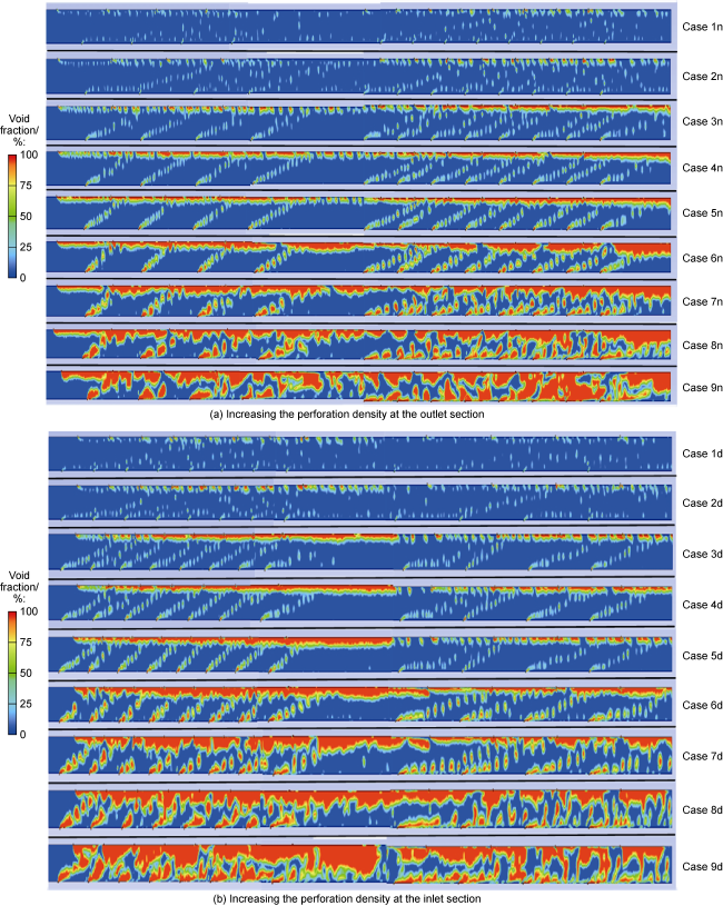
Fig. 5. Flow patterns under two perforation density distribution conditions. Cases 1n-9n represent bubble flow, bubble flow, dispersed bubble-stratified flow, slug-stratified flow, stratified flow, stratified -stratified wave flow, stratified wave flow, stratified wave flow, and stratified wave-annular flow, respectively. Cases 1d-9d represent bubble flow, bubble flow, stratified-dispersed bubble flow, stratified-slug flow, stratified flow, stratified wave-stratified flow, stratified wave flow, stratified wave flow, and annular-stratified wave flow, respectively. |
A comparison of Fig. 5a and Fig. 5b shows that the increased density of perforation in this region will lead to increased air flow, reduced water phase, and increased void fraction. So, the air phase will occupy most of the spaces of the perforated horizontal wellbore. It is noted that the production of horizontal wellbore increases with the increasing perforation density when a single-phase (liquid phase) exists in the wellbore, according to some previous literatures. However, the present work presents that the void fraction increases as the perforation density increases, and such increase will induce a decline of production. In case 9, for example, it was observed that the void fraction increased at the outlet section in case 9n while it increased at the inlet section in case 9d, due to the impact of perforation density distribution. Therefore, the increase of the perforation density at the end sections of the pipe during the two-phase flow will increase the radial air flow rate when the water flow rate kept constant, in other words, the void fraction increases while the holdup fraction decreases. Hence, the production will be affected. Ihara et al. [33] also found that the quantity of oil production in the horizontal wellbore was reduced when the quantity of gases inside the reservoir increased. Under the condition of increasing the perforation density at the outlet section, the increased air flow rate might induce the reverse flow due to pipe wall friction, perforations friction or both. This situation (reverse flow) was observed in case 9n when the pattern was a transition from stratified wave flow to annular flow. Under the condition of increasing the perforation density at the inlet section, this situation above is skipped because of a higher pressure of the axial water flow.
3.2. Comparison between experimental and simulation results
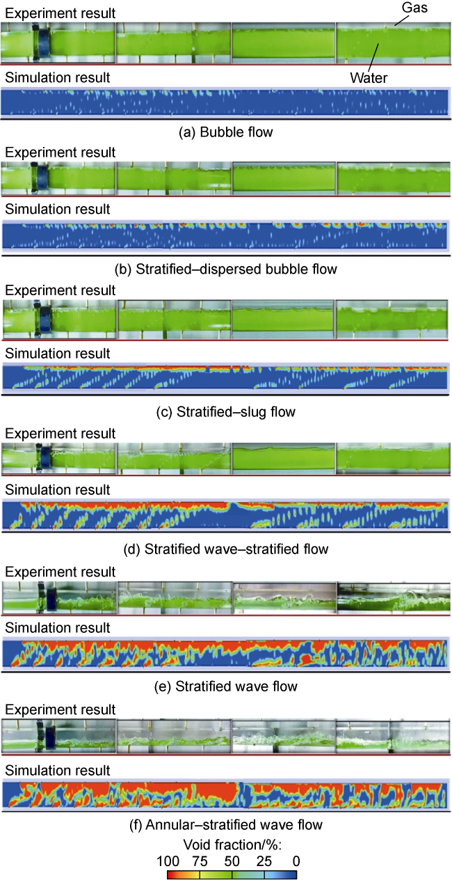
Fig. 6. Comparision of flow patterns in experiment and numerical simulation. |
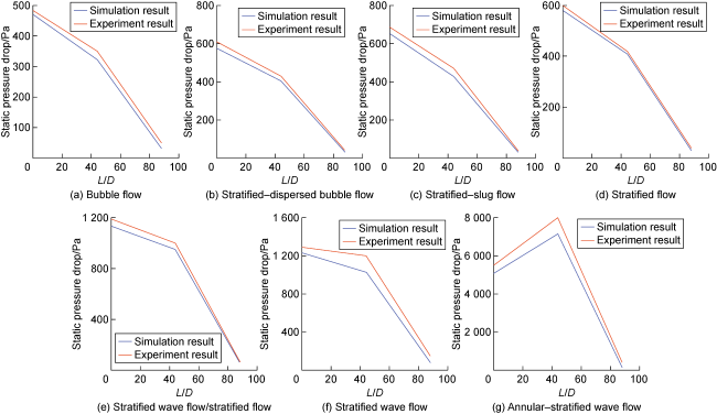
Fig. 7. Comparision of static pressure drop in experiment and numerical simulation. |
Table 1. Comparison of static pressure drop in experiment and simulation |
| Flow pattern | Data source | Static pressure drop at L/D=0/Pa | Static pressure drop at L/D=44/Pa | Static pressure drop at L/D=88/Pa | Average/ Pa | Error/ % |
|---|---|---|---|---|---|---|
| Bubble flow | Experiment | 485 | 350 | 50 | 295 | 6.77 |
| Simulation | 470 | 323 | 32 | 275 | ||
| Stratified-dispersed bubble flow | Experiment | 610 | 430 | 40 | 360 | 6.38 |
| Simulation | 576 | 405 | 31 | 337 | ||
| Stratified-slug flow | Experiment | 685 | 470 | 40 | 398 | 7.28 |
| Simulation | 651 | 427 | 30 | 369 | ||
| Stratified flow | Experiment | 600 | 420 | 40 | 353 | 3.96 |
| Simulation | 580 | 409 | 30 | 339 | ||
| Stratified wave-stratified flow | Experiment | 1 190 | 1 000 | 70 | 753 | 5.17 |
| Simulation | 1 133 | 950 | 60 | 714 | ||
| Stratified wave flow | Experiment | 1 290 | 1 200 | 150 | 880 | 11.36 |
| Simulation | 1 231 | 1 029 | 80 | 780 | ||
| Annular-stratified wave flow | Experiment | 5 500 | 8 000 | 400 | 4 633 | 10.98 |
| Simulation | 5 083 | 7 142 | 150 | 4 125 |
4. Results and discussion
4.1. Distribution of total pressure drop along the perforated horizontal wellbore
Simulation was completed using the ANSYS Fluent to determine the distribution of total pressure drop (the sum of the static pressure drop and the acceleration pressure drop) in each case. Fig. 8 shows the total pressure drop along the perforated horizontal wellbore when the perforation density increases at the outlet section. The total pressure drop was calculated by averaging using the plane cross-section along the perforated horizontal wellbore. In cases 1n to 4n, the curve of the total pressure drop declines sharply. Some fluctuations in the behaviour of the total pressure drop are observed, due to the bubbles generated by the difference in superficial velocity between air and water. In cases 5n to 8n, the total pressure drop variation is normal. From case 1n to case 8n, the total pressure drop increases with the air superficial velocity, while the water superficial velocity is kept constant. This is due to the fact that the total pressure drop is the summation of the static and acceleration pressure drops. When the velocity of the air phase increases, the mixture velocity also increases, leading to an increase in the acceleration pressure drop. The fluctuation in the behaviour of the total pressure drops, which is explained in case 8n, is resulted from the waves generated with the stratified wave flow when the momentum of the air phase is large and the velocity of the water phase is constant (Fig. 8b ).
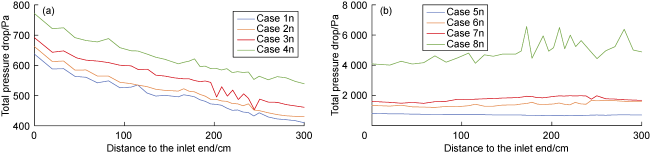
Fig. 8. Total pressure drop in different cases under the condition of increasing the perforation density at the outlet section. |
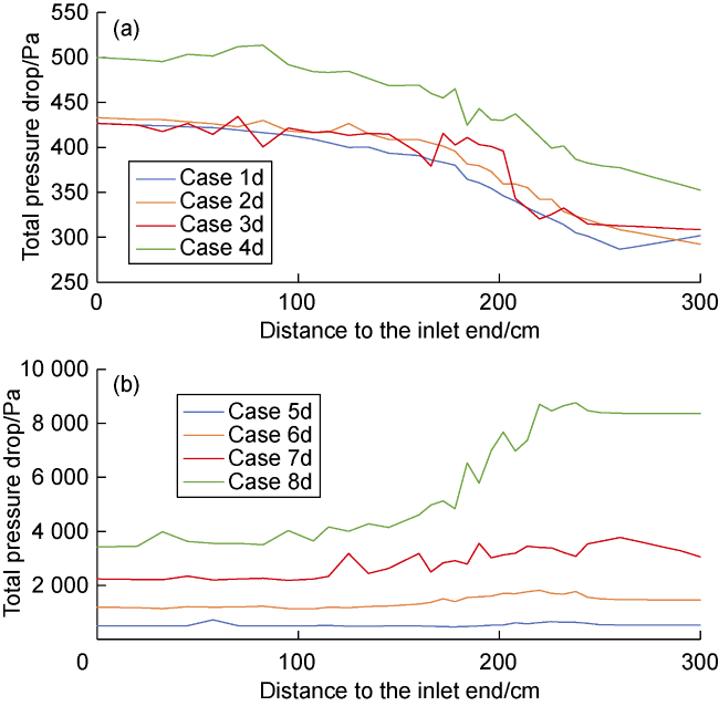
Fig. 9. Total pressure drop in different cases under the condition of increasing the perforation density at the inlet section. |
4.2. Distribution of the mixture superficial velocity along the perforated horizontal wellbore
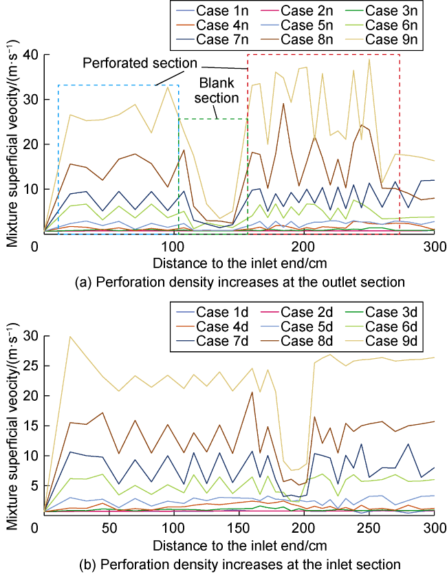
Fig. 10. Distribution of the mixture superficial veocity along the perforated horizontal wellbore in different cases. |
4.3. Distribution of the void fraction along the perforated horizontal wellbore
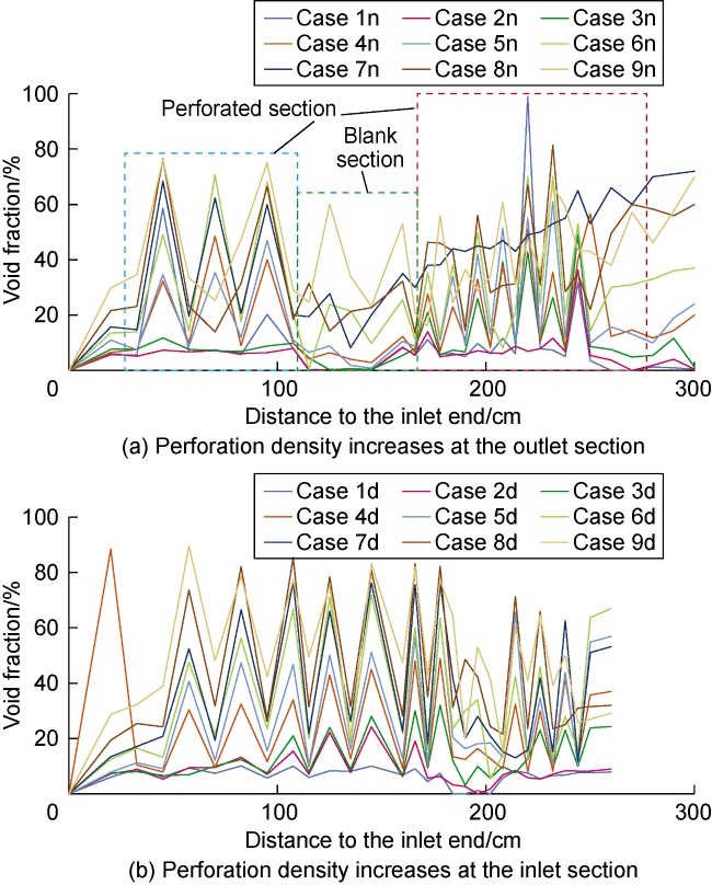
Fig. 11. Distribution of the void fraction along the perforated horizontal wellbore in different cases. |
4.4. Distribution of the liquid film thickness along the perforated horizontal wellbore
According to the simulation with the ANSYS Fluent, the curve of the liquid film thickness fluctulates at similar positions to the curve of the void fraction, but in opposite trend of amplitude, when the perforation density increases at the outlet section of the perforated horizontal wellbore (Fig. 12a ). As per Eq. (1) [34], when the void fraction increases, the liquid film thickness decreases. The liquid film thickness is large and holdup fraction is high in the blank section as it is away from the impact of the radial air flow. Fig. 12b demonstrates that the liquid film thickness behaviour is the opposite of that of Fig. 12a . Hence, in both conditions (the perforation density increases at the inlet and outlet sections of the perforated horizontal wellbore), the liquid film thickness is large in the blank section. When the air flow rate increases, the air phase takes an increasing volume in the perforated horizontal wellbore, allowing the holdup fraction to decrease and thus the liquid film thickness to decrease.
$l=\frac{D}{2}\left( 1-\sqrt{{{\alpha }_{\text{a}}}} \right)$
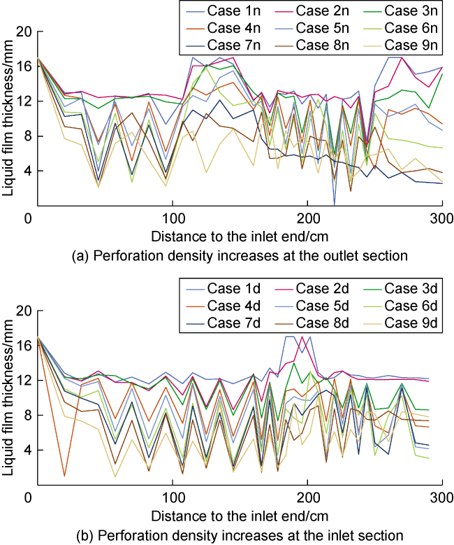
Fig. 12. Distribution of the liquid film thickness along the perforated horizontal wellbore in different cases. |
4.5. Variation of the liquid production of the perforated horizontal wellbore
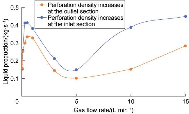
Fig. 13. Relationship of liquid production and gas flow rate. |
The average of the liquid production is 0.228 kg/s when the perforation density increases at the outlet section, and 0.313 kg/s when the perforation density increases at the inlet section. Clearly, the latter is higher. Under the condition of increasing the perforation density at the inlet section, the water flow pressure in the inlet section is high and can overcome the pressure drop resulting from the mixing and friction, thus leading to an increased liquid production.
4.6. Variation of the air production of the perforated horizontal wellbore
The average of the air production is about 0.870 g/s when the perforation density increases at the outlet section of the wellbore, and 0.928 g/s when the perforation density increases at the inlet section of the wellbore. The air production increases with the increasing air flow rate (Fig. 14 ). The air production under the condition of increasing the perforation density at the inlet section is greater than that of the condition of increasing the perforation density at the outlet section.
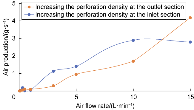
Fig. 14. Air production vs. air flow rate. |
4.7. Normalized liquid flux distribution along the perforated horizontal wellbore
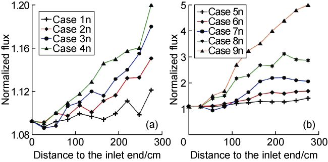
Fig. 15. Normalized liquid flux distribution when the perforation density increases at the outlet section. |
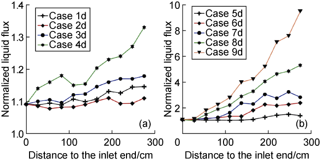
Fig. 16. Normalized liquid flux distribution along the perforated horizontal wellbore when the perforation density increases at the inlet section. |
${{q}_{f}}=\frac{{{q}_{h}}{{L}_{per}}}{{{q}_{T}}}$
5. Conclusions
This study investigated the behaviours of the total pressure drop, air-water superficial velocity, void fraction, liquid film thickness, air and liquid productions with various flow patterns in the perforated horizontal wellbore when the perforation density increases at the inlet and outlet sections, respectively. The results of numerical simulation and experiment were compared to validate the proposed simulation method. It is indicated that the total pressure drop increases with the air flow rate when the water flow rate is kept constant. The mixture superficial velocity fluctuates more violently in the perforated section because of the impact of the radial air flow rate, but it is stable in the unperforated section. When the axial water flow rate is kept constant, the mixture superficial velocity increases as the radial air flow rate increases, and the void fraction increases, the liquid film thickness decreases.
In contrast to the condition of increasing the perforation density at the outlet section, both liquid production and air production increase when the perforation density increases at the inlet section, and the air production increases with the rising air flow rate. The liquid production increases with the bubble flow and begins to decrease at the transition from slug flow to stratified flow. The liquid production increases with the stratified wave flow. The normalized flux of the wellbore when the perforation density increases at the inlet section is greater than that under the condition of the perforation density increased at the outlet section. The normalized flux increases with the radial air flow rate when the axial water flow rate is constant.
Acknowledgement
The authors would like to acknowledge the financial support from the Ministry of Education Malaysia under the Fundamental Research Grant Scheme (FRGS) scheme (20180110FRGS) that enabled the work to be carried out.
Nomenclature
D—average pipe diameter, m;
l—liquid film thickness, m;
L—pipe length, m;
Lper—distance from inlet end, m;
qf—normalized liquid flux;
qh—liquid production per unit length of the perforated section, kg/(s·m);
qT—total liquid production of horizontal wellbore, kg/s;
αa—void fraction, %.