

Introduction
Correlation of oil-bearing strata refers to determine the isochronous correspondence of oil-bearing units (e.g., oil group, sand group, and sub-layer) in different blocks or wells within the oil-bearing strata zone of an oilfield, which belongs to fine stratigraphic correlation [1]. Fine and accurate correlation of oil-bearing strata and high- precision isochronous stratigraphic framework is the foundation and key to realizing reservoir characterization, which is of major significance to predict the spatial distribution of sand bodies, reservoir heterogeneity and favorable oil-bearing zones.
In the development stage of oil and gas fields, there are a large number of development wells (hundreds or even thousands of wells) and oil-bearing layers (tens of layers), so that correlation is a time-consuming work and highly demands geologic expertise and experience, which seriously restricts the correlation efficiency of the oil-bearing strata. Therefore, the study on an automatic correlation method of oil-bearing strata is of vital significance to improve the correlation efficiency and reduce the labor cost.
Previous research on automatic correlation of fine- scale stratigraphy was dated back to the 1970s [2]. Rudman et al. [2] accomplished the correlation between two wells by aligning the logging curves of different lengths through the re-sampling technique and calculating the similarity of the curves, and thus demonstrating the utility of automated computer programs for stratum correlation. Over the past 50 years, scholars all over the world have carried out numerous studies on automatic stratigraphic division and correlation methods. Stratigraphic division and correlation include two processes. First, stratigraphic division in wellbore is carried out based on single-well logging curve data to determine the vertical cycles and evolutionary sequences. Second, inter-well stratigraphic records are traced to establish the stratigraphic correlation among multiple wells. The technologies for single-well analysis include: (1) Signal decomposition such as wavelet transform [3], Walsh transform [4], and spectral analysis [5]. The frequency, amplitude and other characteristics of the logging curves at different scales are picked up to identify singularities, sedimentary cycle interfaces and other markers for stratigraphic division; and (2) Mathematical and statistical methods such as activity function method [6], inner stratigraphic variation method [7], ordered cluster analysis [8], extreme value and variance clustering [9], and fuzzy pattern recognition[10]. Based on interlayer stratigraphic variation and sudden changes of interfaces, etc., statistical analysis is carried out on variance, extreme value to characterize the vertical variation of the electrical characteristics in single wells, based on which the strata in the wells are divided. The primary methods of inter-well tracking include: (1) Mathematical and statistical methods such as correlation analysis [11] and dynamic optimization [12]. The common sub-sequence of the logging curves recorded in different wells is aligned through scale transformations and vertical displacement, and other measures to maximize the characteristic sequence correlation in these wells; (2) Machine learning methods such as clustering analysis [13], self-organizing neural network [14], back propagation neural network [15], and deep neural network [16-17]. Based on a large amount of training data, the numerical statistical features shown by logging curves are extracted and the stratigraphic clustering or division principles are learned by machine, which then are used for correlation of multiple wells.
Existing automatic stratigraphic correlation approaches have attained positive performance on discriminating sedimentary cycles and recognizing stratigraphic interfaces, which tremendously improves the correlation efficiency of stratigraphic division among wells. However, these methods are mostly based on data-driven lithology or cycle correlation, in which the limited stratigraphic regularity features (knowledge) hidden in a large number of database samples are mined. Since the correlation is based on the similarity of the features, it is suitable for correlation of strata that have similar features in the logging curves. For complex strata with rapid changes in lateral sedimentary facies and large differences in thicknesses, the logging curve characteristics of the same stratum are significantly different, so it is impractical to realize isochronous correlation on the basis of lithology and other characteristics through existing methods.
This paper proposes an intelligent automatic correlation method of oil-bearing strata based on pattern constraints (pattern intelligent correlation, PIC in brief). Stratigraphic pattern is introduced into the data-driven algorithm and acts as a knowledge drive to improve correlation precision. Application to many wells in Block Shishen 100 in Shinan Oilfield, Bohai Bay Basin, has proved the practicability of the method for oil-bearing strata correlation.
1. Methodology
In the case of rapid lateral changes of sedimentary facies, especially when the stratum thickness changes greatly at the same time, the automatic correlation process of oil-bearing strata should consider the following two aspects: The marker layer without significant changes in lithology can be automatically correlated on the basis of the feature similarity of the logging curves. However, in the vertical direction of a single well, several layers may be similar to the marker layer, making it difficult to identify the marker layer. For the oil-bearing strata with remarkable changes in lithology due to lateral variation of sedimentary facies, it is difficult to search for comparable information during the automatic correlation process, which may probably lead to diachronism correlation.
To address the two issues above, geologists usually use reliable stratigraphic patterns as constraints. First, they correlate isochronous stratigraphic records including marker layers which are less affected by changes of facies, and then correlate oil-bearing strata that are greatly affected by changes of facies between two adjacent isochronous interfaces.
To realize the automatic correlation of oil-bearing strata according to the above idea, there are two key problems need to be solved: Firstly, when the marker layer is prominent, how to use pattern constraint to improve the correlation accuracy of the marker layer. Secondly, when there is no comparable basis such as a marker layer between two isochronous interfaces, how to use pattern constraints to correlate oil-bearing strata with greatly changing facies to improve the accuracy of automatic correlation of oil-bearing strata among wells. In order to solve the above two key problems, this paper proposes a PIC method that uses geological patterns to constrain the distribution of interfaces between oil-bearing strata, uses a similarity measure machine to identify and correlate the marker layer within the distribution range, and correlates oil-bearing strata between adjacent isochronous interfaces based on an improved dynamic time warping algorithm.
1.1. Geological pattern constraint
In complex situations where lateral sedimentary facies change rapidly and strata thickness differs greatly, the results obtained by automatic correlation of oil-bearing strata generally have some serious errors and are even difficult to comply with geological cognizance. The existent constraint method that defines “stratigraphic interfaces cannot cross” can not improve correlation accuracy. Considering that a stratigraphic pattern reflects the lateral change trend of different oil-bearing strata and can guide inter-well stratigraphic correlation when the lateral sedimentary facies differ rapidly, this paper introduces geological patterns to constrain the automatic correlation of oil-bearing strata.
The essence of pattern constraint is to determine the possible value range of each oil-bearing stratum between two known isochronous interfaces based on the lateral variation law of stratum thickness reflected by the sedimentary pattern. This is to avoid making a wrong judgment on the interface depth that does not comply with the geological law, thereby improving correlation accuracy. According to the pattern, the values of the interface should meet two basic conditions: C1, the lateral change of the stratigraphic interface conforms to the geological pattern; and C2, the lateral change of the stratigraphic thickness conforms to the geological pattern. Strata formed under different geological backgrounds have different patterns, such as aggradational, progradational, retrogradational, etc. This paper takes aggradational pattern as an example to analyze how to define the range of the interface depth that satisfies the two conditions.
The aggradational pattern is characterized by proportional sedimentation, that is, a stratum is in nearly conformable contact with the overlying and underlying strata, and the vertical thickness ratios of all strata are similar laterally. Therefore, taking the thickness of the oil-bearing strata in a standard well (i.e., a well with standard oil-bearing strata) as a reference, the estimated interface depth and the estimated vertical thickness of each oil- bearing stratum in the well to be correlated (i.e., the target well where oil-bearing strata will be divided) are obtained by linear interpolation in proportion. As shown in Fig. 1 a, based on the stratification point and vertical thickness in the standard well, the estimated vertical thickness ${{\hat{d}}_{z}}$ of the oil-bearing stratum ${{o}_{z}}$ and the estimated interface ${{\hat{b}}_{z}}$ between ${{o}_{z-1}}$ and ${{o}_{z}}$ are determined.
Given that the value range of the interface of oil- bearing strata ${{b}_{z}}$ satisfies condition C1 must be an adja-cent interval $\left[ {{{\hat{b}}}_{z}}-{{\delta }_{\text{l},z}}\text{,} \right.$$\left. {{{\hat{b}}}_{z}}+{{\delta }_{\text{r},z}} \right]$ of ${{\hat{b}}_{z}}$ (Fig. 1b ). Assuming that the interval size is positively related to the stratum thickness, that is, the interval radii ${{\delta }_{\text{l},z}}$ and ${{\delta }_{\text{r},z}}$ are variables related to the cumulative thickness of the overlying and the underlying strata, respectively. Then the interval radius can be defined by introducing an interface fluctuation factor θ:
${{\delta }_{\text{l},z}}=\theta \underset{f=1}{\overset{z}{\mathop \sum }}\,{{\hat{d}}_{f}}$
${{\delta }_{\text{r},z}}=\theta \underset{f=z}{\overset{Z+1}{\mathop \sum }}\,{{\hat{d}}_{f}}$
The value range $\left[ {{{\hat{b}}}_{z}}-\theta \underset{f=1}{\overset{z}{\mathop \sum }}\,{{{\hat{d}}}_{f}}, \right.$$\left. {{{\hat{b}}}_{z}}+\theta \underset{f=z}{\overset{Z+1}{\mathop \sum }}\,{{{\hat{d}}}_{f}} \right]$ of the interface of oil-bearing strata ${{b}_{z}}$ that satisfies condition C1 can be obtained. In the equations, Z is the total number of oil-bearing strata; the interface fluctuation factor $\theta \in \left[ 0,1 \right]$, is a hyperparameter determined by standard stratification data. The principle to determine θ is to minimize the value of θ and maximize $P\left\{ b_{z}^{*}\in \left[ {{{\hat{b}}}_{z}}-{{\delta }_{\text{l},z}}\text{ },\text{ }{{{\hat{b}}}_{z}}+{{\delta }_{\text{r},z}} \right] \right\}$ $P\left\{ b_{z}^{*}\in \left[ {{{\hat{b}}}_{z}}-{{\delta }_{\text{l},z}},\text{ }{{{\hat{b}}}_{z}}+{{\delta }_{\text{r},z}} \right] \right\}$.
Considering the constraints of condition C2, the possible value ranges of the interface of adjacent oil-bearing strata are not independent with each other. In some cases, as for a pair of values ${{b}_{z}}={{\hat{b}}_{z}}+{{\delta }_{\text{r},z}}$ and ${{b}_{z+1}}=$ ${{\hat{b}}_{z+1}}-{{\delta }_{\text{l},z+1}}$ from ${{b}_{z}}\in \left[ {{{\hat{b}}}_{z}}-{{\delta }_{\text{l},z}}\text{ },\text{ }{{{\hat{b}}}_{z}}+{{\delta }_{\text{r},z}} \right]$ and ${{b}_{z+1}}\in $ $\left[ {{{\hat{b}}}_{z+1}}-{{\delta }_{\text{l},z+1}},\text{ }{{{\hat{b}}}_{z+1}}+{{\delta }_{\text{r},z+1}} \right]$, the vertical thickness (${{d}_{z}}=$ ${{b}_{z+1}}-{{b}_{z}}={{\hat{b}}_{z+1}}-{{\hat{b}}_{z}}-{{\delta }_{\text{l},z+1}}-{{\delta }_{\text{r},z}}$) of the oil-bearing strata ${{o}_{z}}$ may be extremely small or even negative, so that such a pair of values do not conform to geological cognizance.
Therefore, the possible distribution range $\left[ \left( 1-\varepsilon \right){{{\hat{d}}}_{z}}, \right.$ $\left. \left( 1+\varepsilon \right){{{\hat{d}}}_{z}} \right]$ of the vertical thickness of the oil-bearing strata ${{o}_{z}}$ is defined by introducing the thickness fluctuation factor ε, which constrains the value range of the interface of adjacent oil-bearing strata, so that the value range $\left[ {{{\hat{b}}}_{z}}-{{\delta }_{\text{l},z}}\text{ },\text{ }{{{\hat{b}}}_{z}}+{{\delta }_{\text{r},z}} \right]$ satisfies C1 and C2 at the same time. The thickness fluctuation factor $\varepsilon \in \left[ 0,1 \right]$ is a hyperparameter, which is determined by the thickness data of the standard oil-bearing strata. The principle of determining $\varepsilon $ is to minimize the value of $\varepsilon $ while maxi-mizing $P\left\{ d_{z}^{*}\in \left[ \left( 1-\varepsilon \right){{{\hat{d}}}_{z}},\text{ }\left( 1+\varepsilon \right){{{\hat{d}}}_{z}} \right] \right\}$. The value ranges ${{b}_{z}}$ and ${{b}_{z+1}}$, which meet condition C1, are as the horizontal and vertical coordinates, respectively. The value distribution of two interfaces is shown in orange grid in Fig. 1 c, the condition C2 is used to constrain the joint distribution in the blue area.

Fig. 1 Pattern constraint method for interfaces of oil-bearing strata. |
1.2. Marker layers identification and correlation based on similarity measure machine
The marker layer correlated for oil-bearing strata refer to the isochronous rock layer or lithological interface with distinct features and widely distributed in the stratigraphic profile, which is stable and isochronous within a certain range. The key to identifying and correlating marker layers is to analyze the similarity of electrical characteristics. Existing discrimination methods for feature similarity including cosine similarity, correlation coefficient, Mahalanobis distance, etc. evaluate the signal similarity by comparing the point-to-point error or overall distribution difference of two signals. However, these methods are sensitive to signal noises or local anomalies, and the similarity results from methods for the same signals may be quite different, making it difficult to optimize the evaluation benchmarks for the correlation of marker layers. In recent years, deep learning methods such as contrastive learning have achieved remarkable results in characterizing nonlinear similar features within data and improving noise robustness [18].
Contrastive learning belongs to self-supervised learning, and finishes sample correlation and discrimination by maximizing the similarity of similar samples as well as the difference of heterogeneous samples in the feature space [19]. The typical pattern of contrastive learning usually consists of a proxy task and an objective function. Positive samples and negative samples are defined through the proxy task, and a contrastive loss or contrast function is constructed to optimize the potential representation of the sample in the feature space, so that the characteristics of the sample are as close as possible to the positive sample and as different from negative samples as possible. Contrastive learning technology can achieve data similarity evaluation based on unlabeled data, and has been widely used in fields such as computer vision and natural language processing. The typical algorithms are MoCo (Momentum Contrast) [20], BYOL (Bootstrap Your Own Latent) [21] etc.
This paper proposes a feature similarity measure machine model (SMM) based on the idea of contrast learning, which realizes the self-supervised learning process by constructing a longitudinal contrast learning task among samples, so that it has the ability to extract similar logging features, and conduct automatic identification of marker layers based on the similarity of electrical features.
1.2.1. Construct self-supervised datasets
After intercepting signals of the logging curves from $L$ wells and resampling them to the same length, use the following strategy to construct paired data set for the sampled data.
(1) Randomly select signals from n wells, $s=$ $\left\{ {{x}_{1}},{{x}_{2}},\cdots,{{x}_{n}} \right\}$, use the i-th ($1\le i\le n$) well as a sample well, and perform the following operations on signal ${{x}_{i}}$ from the i-th well.
(2) Select the sub-signal ${{x}_{j}}\left( j=1,\ 2,\ \cdots,\ n \right.$ and $\left. j\ne i \right)$ from a well in s and calculate the root mean square (RMS) error ${{m}_{ij}}$, correlation coefficient ${{r}_{ij}}$ and cosine similarity ${{c}_{ij}}$ between ${{x}_{i}}$ and${{x}_{j}}$. When there exists k that satisfies ${{m}_{ik}}=\underset{j=1,j\ne i}{\overset{n}{\mathop{\min }}}\,\left\{ {{m}_{ij}} \right\}$, ${{r}_{ik}}=\underset{j=1,j\ne i}{\overset{n}{\mathop{\max }}}\,\left\{ {{r}_{ij}} \right\}$, ${{c}_{ik}}=\underset{j=1,j\ne i}{\overset{n}{\mathop{\max }}}\,\left\{ {{c}_{ij}} \right\}$, meaning that the sub-signal ${{x}_{k}}$ from the k-th well and the sub-signal ${{x}_{i}}$ from the i-th well (the sample well) have the minimum error, the maximum correlation coefficient, and the greatest cosine similarity, it is initially assessed that the similarity between ${{x}_{k}}$ and ${{x}_{i}}$ is the largest, and a set of training data $\left\{ \left( {{x}_{i}},{{x}_{j}} \right)\left| j=1,2,\cdots,n \right. \right\}$ is con-structed after manual verification, and meanwhile set a self-supervised label (pseudo-label) ${{t}_{i}}=k$ for it.
(3) Repeat steps (1) and (2) until sufficient datasets are obtained.
1.2.2. SMM
The SMM developed in this paper consists of a residual block, a down-sampling layer and a fully connected layer [22] (Fig. 2 ). Two signals ${{x}_{i}}$ and ${{x}_{j}}$ input for similarity correlation are spliced vertically as $\left[ {{x}_{i}},{{x}_{j}} \right]$, and the residual block, the down-sampling layer and the fully connected layer are executed to output a similarity measure within an interval [0,1]. For a pair of input samples ${{x}_{i}}$ and ${{x}_{j}}$, mark the output of model as ${{y}_{ij}}$. When $j=1,2,\cdots,n$ and$j\ne i$, as determined by the self-supervised label ${{t}_{i}}$, samples ${{x}_{i}}$ and ${{x}_{{{t}_{i}}}}$ have the maximum
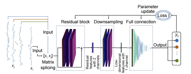
Fig. 2 Architecture of a similarity measure machine (SMM). |
similarity within the group. This means the self-supervision condition $Con{{d}_{i}}$ is established, where the equality sign holds if and only if $j={{t}_{i}}$ (Eq. (3)). When $j=i$, the similarity between samples ${{x}_{i}}$ and ${{x}_{j}}$ should be 1, that is, ${{y}_{ij}}={{y}_{ii}}=1$ is established.
${{y}_{i{{t}_{i}}}}\ge {{y}_{ij}}\text{ }\left( j=1,2,\cdots,n\ \text{and}\ j\ne i \right)$
Next, the SMM model is trained by constructing a contrastive loss function so that its output meets the above two conditions, that is, corresponding to the training dataset for batches B with M sample wells per batch, the training loss of the model is defined as:
$l={{l}_{1}}+{{l}_{2}}$
where ${{l}_{1}}$ is the contrast loss:
${{l}_{1}}=\frac{1}{BM(n-1)}\sum\limits_{b=1}^{B}{\sum\limits_{i=1}^{M}{\sum\limits_{j=1,j\ne i}^{n}{{{\left[ \max \left( 0,{{y}_{ij}}-{{y}_{i{{t}_{i}}}} \right) \right]}^{2}}}}}$
${{l}_{2}}$ is the self-contrasting loss:
${{l}_{2}}=\frac{1}{BM}\sum\limits_{b=1}^{B}{\sum\limits_{i=1}^{M}{{{\left( {{y}_{ii}}-1 \right)}^{2}}}}$
1.2.3. Recognition and correlation of marker layers
When there are multiple logging sections in a single well that have similar characteristics to the marker layer in the standard well, it is difficult to accurately identify the marker layer based only on feature similarity. In this case, pattern constraints need to be introduced. Determine the possible value range (search domain) of the marker layer in the target well (i.e., the well to be correlated) based on the stratigraphic pattern, pick up the logging sub-signals in the range, and input them into the SMM model together with the logging section of the marker layer in the standard well, to complete feature similarity evaluation. Based on the average of the characteristic similarity evaluation results of different well logging curves in the same depth interval, the best matching result is selected as the marker layer in the target well. Taking three wells as an example, we describe the identification process of the marker layer in Fig. 3.
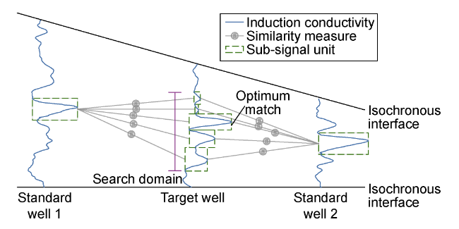
Fig. 3 Principle of automatic correlation of marker layers. |
1.3. Correlation of oil-bearing strata based on dynamic reduction algorithm
The pattern-constrained automatic correlation process of oil-bearing strata between isochronous interfaces involves two key problems: Firstly, how to use the distribution range of interfaces of oil-bearing strata to constrain the correlation process; Secondly, how to use the signal segments that can reflect the characteristics of sedimentary cycles and rhythmic changes as correlation units to weaken the influence of lateral facies changes and avoid lithology correlation based on data points. Many research results show that the conditional dynamic time warping (DTW) algorithm can meet the above two key requirements. Dynamic time warping is a flexible pattern matching algorithm proposed by Itakura [23] in the 1960s. It can match expanded, compressed or deformed patterns and solve the similarity measure of time series of different lengths and classification problems.
The correlation process of oil-bearing strata usually requires comprehensive analysis of logging curves of no less than two standard wells. Although DTW and its improved algorithm have got good results in stratum correlation tasks [24], the method is often suitable for automatic correlation between two wells, that is, one standard well is correlated with the other target well to be correlated. It is not suitable for correlation among multiple wells, because it brings the correlation results with strong partiality.
This paper proposes an N-dimensional dynamic time warping algorithm (NM-DTW) and its conditional form (CNM-DTW). This algorithm accepts the constraints of geological conditions and allows multiple standard wells and multiple logging curves to participate in stratigraphic correlation. The process is effective for dynamic correlation between logging curves of $N-1$ ($N\ge 3$) standard wells and a target well.
1.3.1. NM-DTW
Consider the dynamic time wrap of n wells with m logging curves. The signal set obtained from data preprocessing of the i-th well between two isochronous interfaces is ${{x}_{i}}=\left\{ {{x}_{i,1}},{{x}_{i,2}},\cdots,{{x}_{i,{{Q}_{i}}}} \right\}$, where ${{x}_{i,{{q}_{i}}}}$ is the sub-signal unit of ${{q}_{i}}$(${{q}_{i}}=1,2,\cdots,{{Q}_{i}}$), is composed of m logging curves, and ${{Q}_{i}}$ is the total number of sub-signal units. By constructing a set $G=\left\{ {{x}_{1,{{q}_{1}}-1}},{{x}_{1,{{q}_{1}}}} \right\}\times \left\{ {{x}_{2,{{q}_{2}}-1}},{{x}_{2,{{q}_{2}}}} \right\}\times \cdots \times $ $\left\{ {{x}_{n,{{q}_{n}}-1}},{{x}_{n,{{q}_{n}}}} \right\}$ through Cartesian product, the cumulative wrap loss corresponding to the tuple $g=\left( {{x}_{1,{{q}_{1}}}},{{x}_{2,{{q}_{2}}}},\cdots,{{x}_{n,{{q}_{n}}}} \right)$ composed of ${{q}_{i}}$ sub-signal units can be expressed as:
$D\left( g \right)=d\left( g \right)+\min \left\{ \left. D\left( {{g}'} \right) \right|{g}'\in G,{g}'\ne g \right\}$
where $d(g)=d\left( {{x}_{1,{{q}_{1}}}},{{x}_{2,{{q}_{2}}}},\cdots,{{x}_{n,{{q}_{n}}}} \right)$ is the sub-signal feature similarity distance of $n$ wells, defined as:
$d\left( {{x}_{1,{{q}_{1}}}},\ {{x}_{2,{{q}_{2}}}},\ \cdots,\ {{x}_{n,{{q}_{n}}}} \right)=\sum{\left[ 1-S\left( \alpha,\beta \right) \right]}$
where$\alpha,\beta \in \left\{ {{x}_{1,{{q}_{1}}}},{{x}_{2,{{q}_{2}}}},\cdots,{{x}_{n,{{q}_{n}}}} \right\},\alpha \ne \beta $. S is the feature
similarity evaluation function, calculated by the SMM model above.
Taking the two known isochronous interfaces as the starting and ending points of the dynamic warping algorithm, which means the first signal units of all well logging curves are aligned, namely $D\left( {{x}_{1,1}},\ {{x}_{2,1}},\ \cdots,\ {{x}_{n,1}} \right)=0$, and the last sub-signal units are aligned, the contrast loss of the NM -DTW algorithm can be expressed as
$D\left( {{x}_{1,{{Q}_{1}}}},\ {{x}_{2,{{Q}_{2}}}},\ \cdots,\ {{x}_{n,{{Q}_{n}}}} \right)$.
1.3.2. Conditional search path
The search path defined by the NM-DTW algorithm is $\left\{ 1,2,\cdots,{{Q}_{1}} \right\}\times \left\{ 1,2,\cdots,{{Q}_{2}} \right\}\times \cdots \times \left\{ 1,2,\cdots,{{Q}_{n}} \right\}$ in Cartesian coordinate space, which has algorithmic complexity of $O\left( m\prod\limits_{i=1}^{n}{{{Q}_{i}}} \right)$. Stratigraphic pattern is introduced into the NM-DTW algorithm as a constraint for oil-bearing correlation to reduce the complexity of the algorithm and improves correlation accuracy.
Assuming that the standard well is divided into Z interfaces of oil-bearing strata, the z-th interface of the i-th well falls in the signal interval $\left[ {{u}_{i,z}},{{v}_{i,z}} \right]$. For the standard well, ${{u}_{i,z}}={{v}_{i,z}}$ is given, ${{u}_{i,z}}$ and ${{v}_{i,z}}$ of the target well can be obtained based on the above interface range estimation method. Then the conditional search path can be expressed as: $p={{p}_{1}}\cup {{p}_{2}}$, where ${{p}_{1}}$ refers to the path directly constrained by the condition, and ${{p}_{2}}$ refers to the path indirectly constrained by the condition.
${{p}_{1}}=\bigcup\limits_{z=1}^{Z-1}{\left\{ [{{v}_{1,z}},\ {{u}_{1,z+1}}]\times [{{v}_{2,z}},\ {{u}_{2,z+1}}]\times \cdots \times [{{v}_{n,z}},\ {{u}_{n,z+1}}] \right\}}$
${{p}_{2}}=\bigcup\limits_{z=1}^{Z}{\left\{ [{{u}_{1,z}},\ {{v}_{1,z}}]\times [{{u}_{2,z}},\ {{v}_{2,z}}]\times \cdots \times [{{u}_{n,z}},\ {{v}_{n,z}}] \right\}}$
Taking $n=3$ for example, the conditional search path is shown in Fig. 4. Among them, the search path ${{p}_{2}}$ is constrained by the interval estimate $[{{u}_{i,z}},{{v}_{i,z}}]$ of the interfaces of the same oil-bearing stratum, and search path ${{p}_{1}}$ is constrained by the interval estimate $[{{v}_{i,z}},{{u}_{i,z+1}}]$ of the interface of adjacent oil-bearing strata.
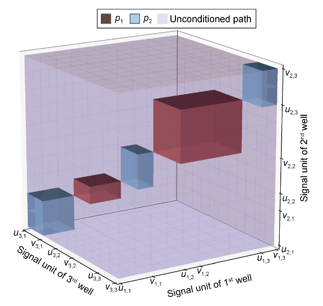
Fig. 4 Search paths of CNM-DTW algorithm. |
1.3.3. Correlate oil-bearing strata
A target well and all standard wells are selected in turn to construct a N-dimensional dynamic time wrap process. The starting and ending points of wrap loss are defined by known adjacent isochronous interfaces as a priori constraint. Conditionalized search paths are based on the distribution of interfaces of oil-bearing strata determined by stratigraphic pattern. Calculate the feature similarity distance d of sub-signal units between the target well and the standard wells, and complete the dynamic iterative process of cumulative wrap loss D, and then find the path that causes the lowest wrap loss, and use the half-amplitude point of the signal unit in the path as the stratigraphic boundary point. Taking three wells as an example, the dynamic correlation and optimal path determination are shown in Fig. 5.
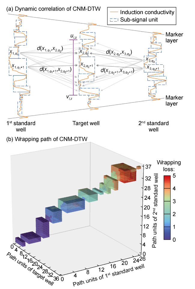
Fig. 5 Correlating oil-bearing strata between isochronous interfaces. |
1.4. PIC procedures
The PIC method involves geological pattern constraint, similarity measure machine and dynamic time warping algorithm, and it consists of the following procedures.
(1) Screening of logging curves and data preprocessing. The logging curves should be able to represent the characteristics of the marker layers, lithological combination and sedimentary cycles, available for all or most wells, and applicable widely. Data preprocessing includes noise reduction, feature transform, morphological filtering, and signal segmentation.
(2) Calculate ${{\hat{b}}_{z}}$ and ${{\hat{d}}_{z}}$ based on the stratigraphic pattern and determine hyperparameters θ and ε in accordance with the standard well data.
(3) Identify marker layers. Construct a self-supervised training dataset, and build and train a machine learning model with the SMM algorithm. Within the distribution range of the interfaces of oil-bearing strata constrained by the stratigraphic pattern, use the trained machine learning model to identify marker layers.
(4) Correlate oil-bearing strata between known isochronous interfaces. Use the distribution range of the interfaces oil-bearing strata to condition the search path of the NM-DTW algorithm and complete the construction of the CNM-DTW algorithm; take the signals reflecting the characteristics of cyclic and rhythmic changes as correlation units to calculate function $d\left( {{x}_{1,{{q}_{1}}}},{{x}_{2,{{q}_{2}}}},\cdots,{{x}_{n,{{q}_{n}}}} \right)$ and loss D of the multi-well with multiple logging curves; search the path corresponding to the lowest loss, and finish stratigraphic correlation according to the path.
2. Case study
Take Shishen 100 block of Bohai Bay Basin as an example to further illustrate the automatic correlation procedures of oil-bearing strata by PIC method and to demonstrate the practicality of the method.
2.1. Geological conditions
The Shishen 100 block is located in the northern part of Shinan Oilfield in Shandong Province, tectonically located in the western part of the central uplift zone of the Dongying Sag in Jiyang Depression that lies in the Bohai Bay Basin, and is a large-scale, nose-shaped structure high in northeast and low in southwest, covering an area of about 46 km2 [25]. The Cenozoic in Dongying Sag is complete, and includes the Quaternary to the Paleocene from the top to the bottom. The Paleocene contains the Dongying Formation, Shahejie Formation, and Kongdian Formation. The Shahejie Formation (Es) is one of the most prominent formations in the Dongying Sag, and can be divided into Es4, Es3, Es2 and Es1 from the top to the bottom. The primary oil pay interval is the middle part of the third member of the Shahejie Formation (oil group), which can be further subdivided into three sand groups of Z1, Z2 and Z3. Z1 and Z2 are the primary oil-bearing sand groups and the target of this study. Z1 is divided top-down into seven sublayers, Z11s, Z11x, Z12, Z13, Z14s, Z14x and Z15; Z2 is divided top-down into Z21s, Z21z, Z21x and Z22.
The study area covers a delta-lake system deposited in a complex and diversified environment, and having a variety of depositional microfacies, such as fan channels, lobes and collapses identified in cores and petrographic calibrations. The top of Z11s and Z14s sublayers, as well as the top and bottom of Z2 sand group have broadly distributed lake-flooding mudstones, which have obvious electrical characteristics such as high natural gamma, high natural potential, high induced conductivity and low resistivity.
2.2. Stratigraphic pattern
The target strata in the study area were deposited in a lake regression system. The thickness of the target layers is different, but regular to some degree, due to the difference in the sedentary amplitude. On the profile in the direction parallel to the source supply, the thickness of the strata becomes thin to different degrees from southeast to northwest (Fig. 6a, 6b ). On the profile in the direction perpendicular to the source supply, the thickness of the strata gradually thins from the middle to the two sides of the study area (Fig. 6a, 6c ). The change trend of the thickness of inner sub-layers is the same as that of the whole target section, and the whole structure shows the pattern of "equal-proportional aggradation". In other words, although the thickness of the same sub-layer varies in different locations (such as Z11x, Z14s, and Z14x), the thickness ratio of the sub-layer to the target interval is close.
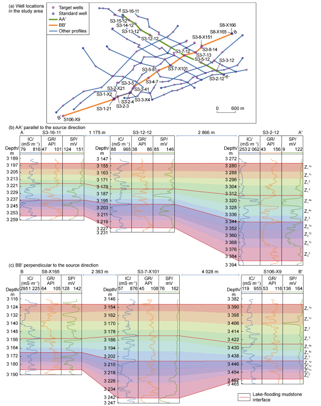
Fig. 6 Well locations in the study area (a), and the change of the thickness of sand groups in the direction parallel to the source direction (b) and perpendicular to the source direction (c). |
2.3. Automatic correlation of oil-bearing strata
This paper takes the AA° profile in Fig. 6 as an example to illustrate the basic correlation steps by using the PIC method. There are 9 wells on this profile, of which 2 wells (S3-16-11 and S3-2-12) are standard wells and the other 7 wells are target wells to be correlated. In the process of correlation, the top and bottom of the target section were known interfaces, and 11 layers between them would be correlated.
(1) Screening of logging curves and data pre-processing. Three logging curves consisting of natural gamma, natural potential and induced conductivity, can well indicate the changes of lithology, sedimentary cycles and other characteristics were selected considering the geological knowledge. Then the logging curves were normalized, and local burr-like noises were removed through morphological filtering technology. Finally, the signals for oil-bearing correlation were extracted through signal decomposition and segmentation.
(2) Mark the oil-bearing strata as ${{o}_{1}}$ to ${{o}_{11}}$ from Z11s to Z22, calculate ${{\hat{b}}_{\text{1}}}$ to ${{\hat{b}}_{11}}$ and ${{\hat{d}}_{1}}$ to ${{\hat{d}}_{11}}$, and determine θ and ε.
(3) Automatic identification of marker layers. Construct 8 000 training datasets (12 pairs of samples per set, and each size of $256\times 1\times 1$), and set the training batches and other parameters; train the SMM model using the adaptive gradient descent algorithm; quantify the logging responses of the marker layers using indicators such as signal amplitude and width, and determine the marker layers to be ${{o}_{5}}$(Z14s) and ${{o}_{8}}$(Z21s). The SMM model was used to identify the marker interfaces near ${{\hat{b}}_{\text{5}}}$ and ${{\hat{b}}_{\text{8}}}$.
(4) Automatic correlation of the other oil-bearing strata. For instance, taking the top of marker layers ${{o}_{5}}$ and ${{o}_{8}}$ as the known isochronous interface, the estimated interfaces ${{\hat{b}}_{6}}$ and ${{\hat{b}}_{7}}$ of oil-bearing strata ${{o}_{6}}$(Z14x) and ${{o}_{7}}$(Z15) were re-determined according to the stratigraphic sedimentary pattern, as well as the estimated thicknesses ${{\hat{d}}_{6}}$ and ${{\hat{d}}_{7}}$. The distribution range of the interface of the oil-bearing strata was updated and the 3D search paths were conditioned to correlate ${{o}_{6}}$ and ${{o}_{7}}$ of target wells by using the CNM-DTW algorithm.
2.4. Analysis and comparisons of correlation performances
Based on python technique, and the method is applied to 13 profiles in the study area, including 24 standard wells and 119 target wells. Fine stratigraphic correlation of the target layers was conducted based on the marker layers, depositional cycles and lithological assemblages by using the strategy of "well-seismic combination, stratigraphic pattern, hierarchical control, and three-dimensional closure". This paper evaluates the effectiveness of the PIC method by taking the artificial correlation results as a reference.
2.4.1. Effectiveness of the PIC method
The practical performance of the method is evaluated from two aspects: the identification effect of marker layers and the correlation effect of oil-bearing strata between marker layers.
(1) The effectiveness of marker layers identification. The similarity measure machine performed excellently in extracting the similarity features. Based on the loss function defined in Eq. (4) and the self-supervised condition set in Eq. (3), the matching rate κ is about 95% and the best is up to 100%, which demonstrated better κ performance of the SMM method than other similar methods such as correlation coefficient, RMS error, and cosine similarity.
$\kappa =\frac{1}{BM}\sum\limits_{b=1}^{B}{\sum\limits_{i=1}^{M}{{{e}_{i}}}}~$
where ${{e}_{i}}$ is a truth function, and it’s 1 when $Con{{d}_{i}}$ is met, or 0 when $Con{{d}_{i}}$ is not met. SMM provides satisfactory identification of marker layers. Based on the logging characteristics, the two interfaces of marker layer in the study area were identified (Fig. 7 ), and the coincidence rate is from the lowest 95.78% to the highest 99.92%. The coincidence rate is defined as:
$R=\sum\limits_{z=1}^{Z}{{{w}_{z}}\frac{\min \{{{b}_{z+1}},b_{z+1}^{*}\}-\max \{{{b}_{z}},b_{z}^{*}\}}{b_{z+1}^{*}-b_{z}^{*}}}$
${{w}_{z}}=\frac{b_{z+1}^{*}-b_{z}^{*}}{\mathop{\sum }_{z=1}^{Z}\left( b_{z+1}^{*}-b_{z}^{*} \right)}$
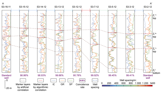
Fig. 7 Marker layers identified on AA′ (the profile location is shown in |
(2) The effect of correlation of oil-bearing strata between marker layers. Based on the CNM-DTW algorithm, the coincidence rate of correlation in the wells drilled through the 13 profiles in the study area reached up to 95.16%, the average coincidence rate reached 90.02%, and the average absolute error of correlation is within 1.14 m. The correlation results of AA° and BB° profiles are excellent, and the average coincidence rate is about 88.70% (Figs. 8 and 9 ).
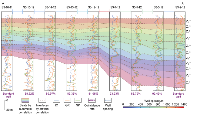
Fig. 8 Correlation of oil-bearing strata on AA′ (the profile location is shown in |
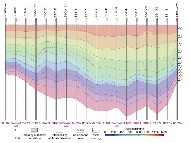
Fig. 9 Oil-bearing strata correlated on BB′ (the profile location is shown in |
However, limited stratigraphic information and constraints bring error to the automatic correlation results. So the correlation accuracy can be improved by increasing data categories or enriching the connotation of constraints, such as introducing depositional boundaries, topographic and geomorphologic control, and consideration of the energy of sedimentary environments.
2.4.2. Comparison of PIC with other automatic correlation methods
DTW (a mathematical statistics method) and PSPNet (a machine learning method) were selected to compare with the PIC method for automatic correlation of oil-bearing strata. DTW is a dynamic time wrap algorithm, which realizes the unconditionalized correlation of logging curves of two wells. PSPNet is an analytic network model for pyramidal scenario, which is an image semantic segmentation method proposed by Zhao et al. [26] in 2017. The pyramid pooling module has an excellent capability of extracting global context information, and provides good results of automatic stratigraphic correlation.
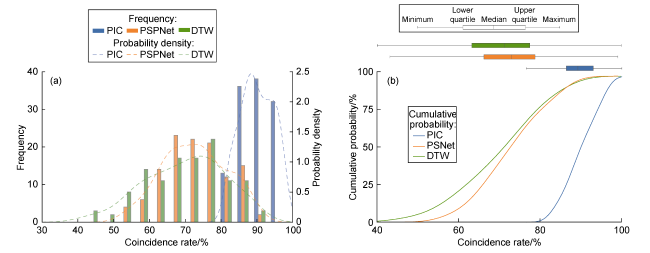
PSPNet and DTW methods were applied to correlate the across-well profiles without constraint from geological pattern. The statistic results of PSPNet, DTW and PIC shown in Fig. 10 show that PIC provides the highest correlation rate, including the minimum, the maximum, and the median values. The distribution probability density function and the cumulative distribution probability function show that the automatic correlation result from the PIC method has a smaller variance of the correlation rate, and the PIC method performs more stably during the process of correlation. The introduction of stratigraphic pattern as a constraint effectively limits the maximum correlation error and reduces the possibility of non-isochronous correlation.
Fig. 10 Correlation results from PIC, PSPNet and DTW. |
The average coincidence rates of PIC, PSPNet and DTW are 90.02%, 72.59% and 69.97%, respectively, indicating the PIC method proposed in this paper is more accurate and practicable than other existing methods.
3. Conclusions
An intelligent automatic correlation method of oil-bearing strata based on pattern constraint is proposed. The automatic correlation process is constrained by stratigraphic sedimentary pattern. It contributes to the solution to stratigraphic correlation under the conditions of rapid lateral sedimentary facies change and large stratigraphic thickness difference. The idea of stratigraphic pattern constraints is introduced into the proposed similarity measure machine algorithm which identifies and correlates the marker layers based on the similarity of electrical features, and effectively improves the accuracy of marker layers correlation. Stratigraphic pattern constraints are applied to an improved conditionally constrained multidimensional multivariate dynamic time warping algorithm which automatically correlates the oil-bearing strata based on multiple standard wells, and effectively improves the accuracy of stratigraphic correlation among the marker layers.
Compared with DTW (a mathematical and statistical algorithm) and PSPNet (a deep learning approach), the PIC method improves the average coincidence rate of automatic correlation from 72.59% to 90.02%, and obtains great application performance.
The PIC method proposed in this paper is suitable for automatic correlation of oil-bearing strata when the stratigraphic sedimentary pattern is clear and reliable, and will be deeply studied in the future for stratigraphic correlation under the conditions of complex geological tectonic backgrounds such as stratigraphic missing and repetition.
Nomenclature
B—training batch, dimensionless;
b—batch number, dimensionless;
${{b}_{z}}$—possible values for the top of the zth oil-bearing stratum, used to store the depth of interface of oil-bearing stratum for automatic correlation, m;
${{\hat{b}}_{z}}$—estimated top interface of the zth oil-bearing stratum obtained by stratigraphic sedimentary patterns, m;
$b_{z}^{*}$—true top interface of the zth oil-bearing stratum, which in the article refers to the correlated stratum top by the geologist, m;
${{C}_{1}}$—condition 1 in pattern constraints;
${{C}_{2}}$—condition 2 in pattern constraints;
${{c}_{ij}}$—cosine similarity of the logging curves from wells i and j, dimensionless;
$Con{{d}_{i}}$—self-supervision condition for well i;
D—wrap loss function, dimensionless;
d—similarity distance function, dimensionless;
${{d}_{z}}$—vertical thickness of the zth oil-bearing stratum, the possible value representing depth, m;
$d_{z}^{*}$—true vertical thickness of the zth oil-bearing stratum, m;
${{\hat{d}}_{z}}$—estimated vertical thickness of the zth oil-bearing stratum, m;
${{\hat{d}}_{f}}$—estimated vertical thickness of overlying or underlying stratum, m;
${{e}_{i}}$—truth function for well i, dimensionless;
f—SN of overlying or underlying oil-bearing stratum, $f=$ $1,2,\cdots,\ Z+1$, dimensionless;
g—polynomial group$\left( {{x}_{1,{{q}_{1}}}},{{x}_{2,{{q}_{2}}}},\cdots,{{x}_{n,{{q}_{n}}}} \right)$, dimensionless;
${g}'$—elements of set $G$, dimensionless;
G—$\left\{ {{x}_{i,{{q}_{i}}-1}},{{x}_{i,{{q}_{i}}}} \right\}$Cartesian product, dimensionless;
i, j—well SN, $i,j=1,2,\cdots,n$, dimensionless;
k—well SN of pseudo-maker, used to derive self-contrasting loss, $k=1,2,\cdots,n$, dimensionless;
l—total loss, dimensionless;
l1—contrast loss, dimensionless;
l2—self-contrast loss, dimensionless;
L—number of wells used in dataset, dimensionless;
M—number of sample wells in a batch of training data, $0<M\le n$, dimensionless;
${{m}_{ij}}$—RMS error of the logging curves from wells i and j;
m—number of logging curves, dimensionless;
n—number of wells randomly selected from L wells, dimensionless;
N—number of dimensions,$N\ge 3$, dimensionless;
${{o}_{z}}$—zth oil-bearing stratum, dimensionless;
O—algorithmic complexity, dimensionless;
p—conditionalized path;
p1—conditional path directly constrained;
p2—conditional path indirectly constrained;
P—Bayesian probability, dimensionless;
${{q}_{i}}$—SN of sub-signal unit of well i, ${{q}_{i}}=1,2,\cdots,{{Q}_{i}}$, dimensionless;
${{Q}_{i}}$—total number of sub-signal units of well i, dimensionless;
${{r}_{ij}}$—correlation coefficient of the logging curves from wells I and j, dimensionless;
R—coincidence rate, dimensionless;
s—set of subsequences, dimensionless;
S—Similarity evaluation function, dimensionless;
${{t}_{i}}$—pseudo-marker of well i, dimensionless;
${{u}_{i,z}}$—left interval of the signal unit of zth oil-bearing stratum in well i, dimensionless;
${{v}_{i,z}}$—right interval of the signal unit of zth oil-bearing stratum in well i, dimensionless;
${{w}_{z}}$—weight of zth oil-bearing stratum, dimensionless;
${{x}_{i}}$—sub-signal of the logging curve from well i, dimensionless;
${{x}_{i,{{q}_{i}}}}$—the qi-th sub-signal unit of well i, dimensionless;
${{y}_{ij}}$—output of the SMM model when wells i and j are input, dimensionless;
z—oil-bearing stratum SN, $z=1,2,\cdots,Z$, dimensionless;
Z—total number of oil-bearing strata, dimensionless;
α—the 1st parameter of similarity evaluation function, dimensionless;
β—the 2nd parameter of similarity evaluation function, dimensionless;
${{\delta }_{\text{l,}z}}$—left radius of the interval adjacent to the interface of zth oil-bearing stratum, m;
${{\delta }_{\text{r},z}}$—right radius of the interval adjacent to the top of zth oil-bearing stratum, m;
ε—thickness fluctuation factor, dimensionless;
θ—interface fluctuation factor, dimensionless;
κ—matching rate, dimensionless;
×—Cartesian product.