

Introduction
With the development of the petroleum industry and the increasing demand for solving complex petroleum engineering challenges, significant attention has been directed toward the study on fluid-solid coupling seepage. During reservoir exploitation, there is a mutual interaction and constraint between fluid seepage and rock deformation. In other words, the seepage and exploitation of oil, gas, and water impacts the redistribution of reservoir stress and the deformation of porous media. The deformation of porous media, in turn, leads to changes in the pore volume within the reservoir, resulting in alterations in reservoir physical properties, especially porosity and permeability. These changes, in a feedback loop, subsequently affect the seepage and exploitation of reservoir fluids. The stress field is coupled with the seepage field, with permeability serving as a “bridge” between them and also the key for achieving a truly integrated fluid-solid coupling analysis.
The dynamic permeability model serves as the foundation for fluid-solid coupling analysis. Researchers both domestically and internationally have extensively explored this topic, proposing numerous models. These models can be categorized into two types based on independent variables. The first type characterizes the relationship between permeability and either pore pressure or effective stress [1-2]. From a functional perspective, they fall into categories such as power model, exponential model, binomial model, and logarithmic model [3]. These models are derived from the deformation of structures such as flat fractures, circular tube bundles, elliptical tube bundles, and star-like tube bundles based on the hypothesis of uniaxial strain. Under the assumption of constant overburden pressure [4], dynamic permeability can be directly calculated as pore pressure changes and can be extensively used in traditional reservoir numerical simulation [5] and well testing interpretation [6]. The second type characterizes the relationship between permeability and porosity, resulting in various equations that link permeability with other parameters like porosity, particle radius, specific surface area, and tortuosity based on the Kozeny-Carman equation [7⇓-9]. Therefore, the relationship between permeability and volumetric strain can be obtained due to the direct and clear relationship between porosity and volumetric strain during rock deformation [10]. As the understanding of the fluid-solid coupling deformation process deepens, it has become evident that the surrounding rocks outside the reservoir exert a constraining effect on deformation. Furthermore, there is a significant error in the assumptions of constant overburden pressure and uniaxial deformation [11]. Fluid-solid coupling calculations have gradually developed into mechanical calculations, where stress, strain, and displacement fields are determined using a volume much larger than the seepage area. Subsequently, dynamic physical parameters are deduced based on the mechanical calculation results [12⇓-14]. The second type of dynamic permeability models, represented by the Kozeny-Carman equation, has gained widespread use in modern geomechanical calculations due to its compliance with the theoretical basis of three-dimensional deformation [15-16].
The dynamic permeability models discussed earlier are all scalar models, neglecting the consideration of the anisotropy of permeability and the anisotropy of rock deformation degree. However, the anisotropy of permeability has been widely recognized in the field of seepage [17-18]. Additionally, distinct directions exhibit significant differences in deformation degrees during the development of oil and gas reservoirs [19]. Therefore, the investigation of anisotropic dynamic permeability holds crucial practical significance. Li et al. [20] and Daigle et al. [21] described the anisotropy of permeability using the concept of anisotropic tortuosity. At the macro scale, however, the key parameters in their models are typically considered as constants, which limit their ability to characterize the changes in permeability in various directions during deformation. Wang et al. [22] transformed the equation for volumetric strain into a weighted sum of three normal strains based on the Kozeny-Carman equation. They employed different weights to calculate vertical and horizontal permeability but did not provide a strict theoretical basis for the selection of weights. Thus, it is evident that despite the attention given to the issue of anisotropic dynamic permeability, a reasonable and reliable model has not yet been fully developed. In this paper, based on the tortuous capillary network model, a direct relational expression between anisotropic permeability and rock normal strain was established through theoretical derivation. Meanwhile, the model was verified through pore-scale flow simulations, presenting an effective approach for implementing fluid-solid coupling numerical simulation.
1. Basic principle
Before deformation analysis, it is necessary to define the concept of stress. Stress refers to the internal force exerted on a unit area, signifying the distribution of these internal forces. Therefore, the concept of stress must be explicitly associated with its corresponding area. Firstly, we define the area corresponding to the frame stress as the apparent area of the rock rather than the frame area itself. Rock frame stress is defined as the average stress of frame internal forces over the apparent area of the rock:
${{\sigma }_{ij}}=\left( 1-\phi \right){{\sigma }_{s,ij}}$
As this paper primarily focuses on the changes compared to the initial state, the initial state is considered as the zero point of stress and strain.
Based on the above definition, the total stress at any cross-section within the rock can be expressed as follows [23]:
${{\sigma }_{t,ij}}={{\sigma }_{ij}}-\phi \Delta p{{\delta }_{ij}}$
The apparent strain of the rock is defined as below:
${{\varepsilon }_{ij}}=\frac{1}{2}\left( \frac{\partial {{u}_{i}}}{\partial {{x}_{j}}}+\frac{\partial {{u}_{j}}}{\partial {{x}_{i}}} \right)$
The apparent volumetric strain of the rock refers to the sum of three apparent normal strains, as expressed in Eq. (4) below:
$\varepsilon ={{\varepsilon }_{x}}+{{\varepsilon }_{y}}+{{\varepsilon }_{z}}$
Based on the linear elastic isotropic porous media, the constitutive equation can be expressed as follows [23]:
${{\sigma }_{t,ij}}=2G{{\varepsilon }_{ij}}+\frac{2G\nu }{1-2\nu }{{\delta }_{ij}}\varepsilon -\left( 1-\frac{{{M}_{p}}}{{{M}_{s}}} \right){{\delta }_{ij}}\Delta p$
By substituting Eq. (2) into Eq. (5), the frame stress can be acquired:
${{\sigma }_{ij}}=2G{{\varepsilon }_{ij}}+\frac{2G\nu }{1-2\nu }{{\delta }_{ij}}\varepsilon -\left( 1-\phi -\frac{{{M}_{\text{p}}}}{{{M}_{\text{s}}}} \right){{\delta }_{ij}}\Delta p$
For frame particles, the constitutive equation of linear elastic isotropic materials is [23]:
${{\sigma }_{s,ij}}=2{{G}_{s}}{{\varepsilon }_{s,ij}}+\frac{2{{G}_{s}}{{\nu }_{s}}}{1-2{{\nu }_{s}}}{{\delta }_{ij}}{{\varepsilon }_{\text{s}}}$
According to Eq. (7), three normal strains of the rock frame can be integrated as follows:
${{\varepsilon }_{\text{s},i}}=\frac{\left( 1+{{\nu }_{\text{s}}} \right){{\sigma }_{\text{s},i}}-{{\nu }_{\text{s}}}\left( {{\sigma }_{\text{s},x}}+{{\sigma }_{\text{s},y}}+{{\sigma }_{\text{s},z}} \right)}{3{{M}_{\text{s}}}\left( 1-2{{\nu }_{\text{s}}} \right)}$
The following equation can be obtained by substituting Eq. (1) and Eq. (6) into Eq. (8):
${{\varepsilon }_{\text{s},i}}=\frac{\frac{2G\left[ (1+{{\nu }_{\text{s}}}){{\varepsilon }_{i}}-{{\nu }_{\text{s}}}\varepsilon \right]}{1-2{{\nu }_{\text{s}}}}+\frac{2G\nu \varepsilon }{1-2\nu }-\left( 1-\phi -\frac{{{M}_{\text{p}}}}{{{M}_{\text{s}}}} \right)\Delta p}{3{{M}_{\text{s}}}\left( 1-\phi \right)}$
The volumetric strain of the rock frame represents the sum of three frame normal strains, which can be written as follows:
${{\varepsilon }_{\text{s}}}={{\varepsilon }_{\text{s},x}}+{{\varepsilon }_{\text{s},y}}+{{\varepsilon }_{\text{s},z}}$
By substituting Eq. (9) into Eq. (10), Eq. (11) can be acquired:
${{\varepsilon }_{\text{s}}}=\frac{{{M}_{\text{p}}}\varepsilon -\left( 1-\phi -\frac{{{M}_{\text{p}}}}{{{M}_{\text{s}}}} \right)\Delta p}{{{M}_{\text{s}}}\left( 1-\phi \right)}$
2. Dynamic porosity model
The dynamic porosity of the rock is determined by both the apparent deformation of the rock and the deformation of the rock frame. Fig. 1 illustrates the variation relationship between pore volume, frame volume, and apparent volume during rock deformation. According to Fig. 1a , Eq. (12) can be derived:
${{\phi }_{0}}=\frac{{{V}_{0}}-{{V}_{s0}}}{{{V}_{0}}}$
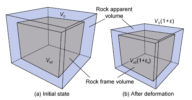
Fig. 1 Schematic diagram of pore volume changes during rock deformation. |
According to Fig. 1b , Eq. (13) can be derived:
$\phi =\frac{{{V}_{0}}\left( 1+\varepsilon \right)-{{V}_{s0}}\left( 1+{{\varepsilon }_{s}} \right)}{{{V}_{0}}\left( 1+\varepsilon \right)}$
Then, the dynamic porosity of the rock can be expressed as Eq. (14) by substituting Eq. (12) into Eq. (13):
$\phi =1-\frac{\left( 1-{{\phi }_{0}} \right)\left( 1+{{\varepsilon }_{\text{s}}} \right)}{\left( 1+\varepsilon \right)}$
The reservoir rock experiences both internal stress from the fluid in the pores and external stress exerted by the overburden rock. When the pore pressure decreases, there are two mechanisms of particle expansion and compaction of rock frame, and the rock frame, pores, and apparent volume respond accordingly. Previous experiments have indicated that the particle expansion is a secondary factor. When there is a decrease in pore pressure, the failure of the fluid to resist the overburden pressure leads to additional compression of the formation.
$\phi =\frac{\varepsilon +{{\phi }_{0}}}{1+\varepsilon }$
Eq. (15) represents the relationship between porosity and volumetric strain established by Ran et al. [10].
3. Anisotropic dynamic permeability model
In the 1920s to 1950s, Kozeny and Carman formulated the relational expression between permeability and porosity of porous media, giving rise to the widely accepted Kozeny-Carman equation. Initially, this equation derived the relational expression between permeability and porosity and specific surface area based on the capillary bundle model. Subsequently, the specific surface area equation of the spherical particle model was incorporated, resulting in the most commonly used relationship between permeability and porosity [7]:
$K=\frac{{{D}^{2}}}{72{{\tau }^{2}}}\frac{{{\phi }^{3}}}{{{\left( 1-\phi \right)}^{2}}}$
In the context that the frame particle deformation is ignored during rock deformation, the following equation can be obtained by substituting Eq. (15) into Eq. (16) [10]:
$\frac{K}{{{K}_{0}}}=\frac{{{\left( {{\phi }_{0}}+\varepsilon \right)}^{3}}}{\phi _{0}^{3}\left( 1+\varepsilon \right)}$
Eq. (17) directly establishes the relationship between permeability and volumetric strain, providing a straightforward and widely employed method in fluid-solid coupling calculations. It partially reflects the influence and coupling effects of deformation fields on seepage fields. However, this equation does have limitations in the following two aspects. (1) The pore structure of rock is characterized by anisotropy, existing significant differences, especially in permeability between the vertical and horizontal directions, so it is clearly inconsistent with reality to use a unified relational expression to describe the fluid-solid coupling characteristics. (2) During deformation of the rock, strains in different directions demonstrate significant difference. Mostly, the vertical strain is notably greater than the plane strain [19]. In this case, the changes in permeability in all directions differ inevitably, so it is inaccurate to characterize their changes with a unified relational expression. Hence, in fluid-solid coupling analysis, it becomes imperative to consider anisotropic changes in permeability and establish relational expression between permeability in each direction and normal strain to accurately reflect the impact of distinct deformation fields on the seepage field. As a result, three normal strains were taken as the basic variables to establish a relational expression between permeability and rock deformation.
The analysis was carried out based on the capillary network model. Considering the coordinate system depicted in Fig. 2 , the principal values of the permeability tensor (Kx, Ky, Kz) and normal strain (εx, εy, εz) share the same direction. To illustrate the analysis, the x direction was undertaken as an example:
The Poiseuille equation for a single capillary is given as follows [7]:
$q=\frac{\pi {{r}_{x}}^{4}}{8\mu }\frac{\Delta p}{{{l}_{x}}}$
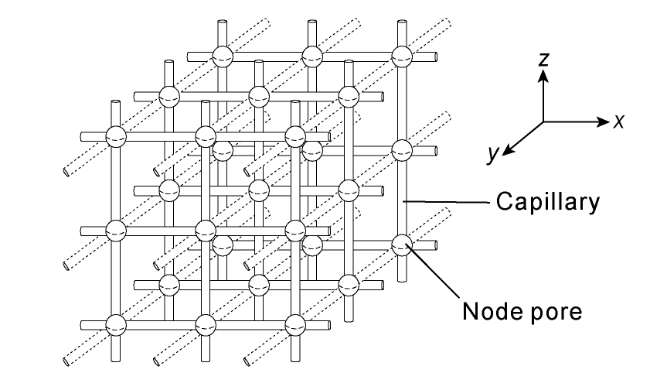
Fig. 2 Schematic diagram of the capillary network model. |
The number of capillaries per y-z cross-section is calculated with the equation below:
$N=\frac{{{\phi }_{x}}{{L}_{x}}}{\pi {{r}_{x}}^{2}{{l}_{x}}}$
where ${{\phi }_{x}}$is the effective porosity of the flow in x direction, referring to the ratio of the pore volume with a non-zero flow velocity during displacement along x direction to the apparent volume of the rock. It is important to note that not all connected pores contribute to seepage in a given direction. In other words, not all connected pores facilitate flow during displacement in a particular direction, and pores with a flow velocity of 0 may not necessarily be the same during displacement in different directions. Consequently, the effective porosity was introduced for the seepage in a specific direction.
According to the definition of permeability, the following equation can be obtained:
${{K}_{x}}=\frac{qAN\mu {{L}_{x}}}{A\Delta p}$
After Eq. (18) and Eq. (19) are substituted into Eq. (20), the following equation can be obtained:
${{K}_{x}}=\frac{{{\phi }_{x}}{{r}_{x}}^{2}}{8{{\tau }_{x}}^{2}}$
where ${{\tau }_{x}}$ is the capillary tortuosity in x direction, referring to the ratio of the true capillary length during flowing in x direction to the apparent length of the rock in this direction. Thus, the initial permeability is:
${{K}_{x0}}=\frac{{{\phi }_{x0}}{{r}_{x0}}^{2}}{8{{\tau }_{x0}}^{2}}$
Therefore, the ratio of permeability in x direction before and after deformation is expressed as follows:
$\frac{{{K}_{x}}}{{{K}_{x0}}}=\frac{{{\phi }_{x}}}{{{\phi }_{x0}}}\frac{{{r}_{x}}^{2}}{{{r}_{x0}}^{2}}\frac{{{\tau }_{x0}}^{2}}{{{\tau }_{x}}^{2}}$
In any determined area, the number of capillaries remains constant before and after deformation. According to Eq. (19), the following equation can be obtained:
$\frac{{{\phi }_{x}}}{{{\phi }_{x0}}}=\frac{{{r}_{x}}^{2}{{l}_{x}}{{L}_{x0}}}{{{L}_{x}}{{r}_{x0}}^{2}{{l}_{x0}}}=\frac{{{r}_{x}}^{2}{{\tau }_{x}}}{{{r}_{x0}}^{2}{{\tau }_{x0}}}$
Substituting Eq. (24) into Eq. (23), the following equation can be acquired:
$\frac{{{K}_{x}}}{{{K}_{x0}}}=\frac{{{r}_{x}}^{4}}{{{r}_{x0}}^{4}}\frac{{{\tau }_{x0}}}{{{\tau }_{x}}}$
The truly curved capillary displayed in Fig. 3a can be equivalent to the inclined straight capillary in Fig. 3c according to its length. If the bending direction of the effective tortuous capillary flowing in x direction is uniformly distributed in y and z directions, the angle between the projection OB of the equivalent inclined straight capillary onto the yOz plane and the coordinate axis is denoted as $\angle HOB=\angle GOB={\pi }/{4}\;$.
According to Fig. 3 d, the following equation can be obtained:
${{l}_{x}}^{2}={{L}_{x}}^{2}+{{w}^{2}}={{\left[ {{L}_{x0}}\left( 1+{{\varepsilon }_{x}} \right) \right]}^{2}}+{{\left[ {{w}_{0}}\left( 1+{{\varepsilon }_{OB}} \right) \right]}^{2}}$
${{w}_{0}}=\sqrt{{{l}_{x0}}^{2}-{{L}_{x0}}^{2}}$
By referring to the basic theory of elastic mechanics, the normal strain ${{\varepsilon }_{i}}$ in i direction causes a linear strain ${{\varepsilon }_{i}}{{\cos }^{2}}\alpha $ in the direction with an angle α with the i direction. Combined with the superposition principle, the following equation can be obtained:
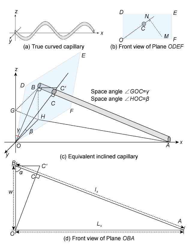
Fig. 3 Equivalent schematic diagram of tortuous capillary tube. |
${{\varepsilon }_{OB}}={{\varepsilon }_{x}}{{\cos }^{2}}\frac{\pi }{2}+{{\varepsilon }_{y}}{{\cos }^{2}}\frac{\pi }{4}+{{\varepsilon }_{z}}{{\cos }^{2}}\frac{\pi }{4}=\frac{{{\varepsilon }_{y}}+{{\varepsilon }_{z}}}{2}$
After incorporating the Eq. (27) and Eq. (28) into Eq. (26), a new expression could be written as follows:
${{l}_{x}}^{2}={{\left[ {{L}_{x0}}\left( 1+{{\varepsilon }_{x}} \right) \right]}^{2}}+\left( {{l}_{x0}}^{2}-{{L}_{x0}}^{2} \right){{\left[ 1+{\left( {{\varepsilon }_{y}}+{{\varepsilon }_{z}} \right)}/{2}\; \right]}^{2}}$
Therefore, the ratio of tortuosity before and after deformation can be expressed as follows:
$\frac{{{\tau }_{x}}}{{{\tau }_{x0}}}=\frac{{{l}_{x}}}{{{L}_{x0}}\left( 1+{{\varepsilon }_{x}} \right){{\tau }_{x0}}}=$ $\frac{\sqrt{{{\left( 1+{{\varepsilon }_{x}} \right)}^{2}}+\left( {{\tau }_{x0}}^{2}-1 \right){{\left[ 1+\left( {{\varepsilon }_{y}}+{{\varepsilon }_{z}} \right)/2 \right]}^{2}}}}{\left( 1+{{\varepsilon }_{x}} \right){{\tau }_{x0}}}$
The change in capillary radius is definitively influenced by the area strain of the Plane ODEF, which represents the cross-section perpendicular to the capillary. The area strain is the sum of two perpendicular linear strains, namely:
${{\varepsilon }_{\text{A}x}}={{\varepsilon }_{OC}}+{{\varepsilon }_{NM}}$
For the strain in the OC direction, the following equation can be obtained according to Fig. 3c and 3d:
${{\varepsilon }_{OC}}={{\varepsilon }_{x}}{{\cos }^{2}}\alpha +{{\varepsilon }_{y}}{{\cos }^{2}}\beta +{{\varepsilon }_{z}}{{\cos }^{2}}\gamma $
Considering auxiliary point C°, the following equation can be obtained:
$\cos \beta =\cos \gamma =\frac{OG}{O{C}'}=\frac{OG\sin \alpha }{OB}=\frac{\sin \alpha }{\sqrt{2}}$
Moreover, the following equation can be obtained by substituting Eq. (33) into Eq. (32):
${{\varepsilon }_{OC}}={{\varepsilon }_{x}}{{\cos }^{2}}\alpha +\frac{{{\varepsilon }_{y}}+{{\varepsilon }_{z}}}{2}{{\sin }^{2}}\alpha $
Regarding the strain in the NM direction, since NM is in the Plane ODEF and perpendicular to OC, it can be seen from the geometric relationship that NM is perpendicular to the Plane OBA, then it is parallel to GH. Therefore ${{\varepsilon }_{NM}}={{\varepsilon }_{GH}}$, the following equation can be obtained:
${{\varepsilon }_{NM}}={{\varepsilon }_{x}}{{\cos }^{2}}\frac{\pi }{2}+{{\varepsilon }_{y}}{{\cos }^{2}}\frac{\pi }{4}+{{\varepsilon }_{z}}{{\cos }^{2}}\frac{\pi }{4}=\frac{{{\varepsilon }_{y}}+{{\varepsilon }_{z}}}{2}$
After Eq. (34) and Eq. (35) are substituted into Eq. (31), the area strain of the Plane ODEF can be acquired:
${{\varepsilon }_{Ax}}={{\varepsilon }_{x}}{{\cos }^{2}}\alpha +\frac{{{\varepsilon }_{y}}+{{\varepsilon }_{z}}}{2}{{\sin }^{2}}\alpha +\frac{{{\varepsilon }_{y}}+{{\varepsilon }_{z}}}{2}$
According to Fig. 3d , the following equation can be obtained:
$\sin \alpha =\frac{{{L}_{x}}}{{{l}_{x}}}=\frac{1}{{{\tau }_{x}}}$
Therefore, Eq. (36) can be transformed into Eq. (38):
${{\varepsilon }_{Ax}}={{\varepsilon }_{x}}\left( 1-\frac{1}{{{\tau }_{x}}^{2}} \right)+\frac{{{\varepsilon }_{y}}+{{\varepsilon }_{z}}}{2}\left( 1+\frac{1}{{{\tau }_{x}}^{2}} \right)$
During the rock deformation process, ${{\tau }_{x}}$ will continue to change dynamically, so Eq. (38) contains a nonlinear coefficient. Considering that the rock deformation is small, Eq. (38) is linearized using ${{\tau }_{x0}}$, and we can get:
${{\varepsilon }_{Ax}}={{\varepsilon }_{x}}\left( 1-\frac{1}{{{\tau }_{x0}}^{2}} \right)+\frac{{{\varepsilon }_{y}}+{{\varepsilon }_{z}}}{2}\left( 1+\frac{1}{{{\tau }_{x0}}^{2}} \right)$
Similarly, the area strain of the rock frame in the Plane ODEF can be obtained as follows:
${{\varepsilon }_{s,Ax}}={{\varepsilon }_{s,x}}\left( 1-\frac{1}{{{\tau }_{x0}}^{2}} \right)+\frac{{{\varepsilon }_{s,y}}+{{\varepsilon }_{\text{s},z}}}{2}\left( 1+\frac{1}{{{\tau }_{x0}}^{2}} \right)$
In any study area, the capillary number within that area is constant before and after deformation, and the ratio of pore areas in the cross-section is considered as the ratio of capillary cross-sectional areas:
$\frac{{{r}_{x}}^{2}}{{{r}_{x0}}^{2}}=\frac{\left( 1+{{\varepsilon }_{\text{A}x}} \right)-\left( 1-{{\phi }_{\text{A}x}} \right)\left( 1+{{\varepsilon }_{s,\text{A}x}} \right)}{{{\phi }_{\text{A}x}}}$
where ${{\phi }_{\text{A}x}}$ represents the effective surface porosity of the cross-section perpendicular to the capillary seepage in x direction, but it is not the effective porosity. Taking Fig. 2 as an example, ${{\phi }_{\text{A}x}}$ refers to the surface porosity of the x direction capillary in the cross-section perpendicular to the capillary which seepage in x direction. It is worth mentioning that node pores may not contribute to the effective surface porosity, which means that the value of the effective surface porosity should be less than or equal to the effective porosity.
Substituting Eqs. (30) and (41) into (25), a new expression is obtained:
$\frac{{{K}_{x}}}{{{K}_{x0}}}=\frac{{{\left[ \left( 1+{{\varepsilon }_{\text{A}x}} \right)-\left( 1-{{\phi }_{\text{A}x}} \right)\left( 1+{{\varepsilon }_{\text{s},\text{A}x}} \right) \right]}^{2}}\left( 1+{{\varepsilon }_{x}} \right){{\tau }_{x0}}}{{{\phi }_{\text{A}x}}^{2}\sqrt{{{\left( 1+{{\varepsilon }_{x}} \right)}^{2}}+\left( {{\tau }_{x0}}^{2}-1 \right){{\left[ 1+\left( {{\varepsilon }_{y}}+{{\varepsilon }_{z}} \right)/2 \right]}^{2}}}}$
Eq. (42) shows the relationship between the permeability in x direction and the normal strain of the rock. Similarly, the dynamic permeability in y and z directions can be expressed as Eq. (43) and (44), respectively:
$\frac{{{K}_{y}}}{{{K}_{y0}}}=\frac{{{\left[ \left( 1+{{\varepsilon }_{Ay}} \right)-\left( 1-{{\phi }_{Ay}} \right)\left( 1+{{\varepsilon }_{s,Ay}} \right) \right]}^{2}}\left( 1+{{\varepsilon }_{y}} \right){{\tau }_{y0}}}{{{\phi }_{Ay}}^{2}\sqrt{{{\left( 1+{{\varepsilon }_{y}} \right)}^{2}}+\left( {{\tau }_{y0}}^{2}-1 \right){{\left[ 1+\left( {{\varepsilon }_{x}}+{{\varepsilon }_{z}} \right)/2 \right]}^{2}}}}$
$\frac{{{K}_{z}}}{{{K}_{z0}}}=\frac{{{\left[ \left( 1+{{\varepsilon }_{Az}} \right)-\left( 1-{{\phi }_{Az}} \right)\left( 1+{{\varepsilon }_{\text{s},Az}} \right) \right]}^{2}}\left( 1+{{\varepsilon }_{z}} \right){{\tau }_{z0}}}{{{\phi }_{Az}}^{2}\sqrt{{{\left( 1+{{\varepsilon }_{z}} \right)}^{2}}+\left( {{\tau }_{z0}}^{2}-1 \right){{\left[ 1+\left( {{\varepsilon }_{x}}+{{\varepsilon }_{y}} \right)/2 \right]}^{2}}}}$
where
$\left\{ \begin{align} & {{\varepsilon }_{\text{A}y}}={{\varepsilon }_{y}}\left( 1-\frac{1}{{{\tau }_{y0}}^{2}} \right)+\frac{{{\varepsilon }_{x}}+{{\varepsilon }_{z}}}{2}\left( 1+\frac{1}{{{\tau }_{y0}}^{2}} \right) \\ & {{\varepsilon }_{s,\text{A}y}}={{\varepsilon }_{s,y}}\left( 1-\frac{1}{{{\tau }_{y0}}^{2}} \right)+\frac{{{\varepsilon }_{s,x}}+{{\varepsilon }_{s,z}}}{2}\left( 1+\frac{1}{{{\tau }_{y0}}^{2}} \right) \\ & {{\varepsilon }_{\text{A}z}}={{\varepsilon }_{z}}\left( 1-\frac{1}{{{\tau }_{z0}}^{2}} \right)+\frac{{{\varepsilon }_{x}}+{{\varepsilon }_{y}}}{2}\left( 1+\frac{1}{{{\tau }_{z0}}^{2}} \right) \\ & {{\varepsilon }_{\text{s},\text{A}z}}={{\varepsilon }_{\text{s},z}}\left( 1-\frac{1}{{{\tau }_{z0}}^{2}} \right)+\frac{{{\varepsilon }_{\text{s},x}}+{{\varepsilon }_{\text{s},y}}}{2}\left( 1+\frac{1}{{{\tau }_{z0}}^{2}} \right) \\ \end{align} \right.$
If the strain of the rock frame is ignored, the anisotropic dynamic permeability model (ADPM) can be simplified as follows, which is a function of normal strain:
$\left\{ \begin{align} & \frac{{{K}_{x}}}{{{K}_{x0}}}=\frac{{{\left( {{\varepsilon }_{\text{A}x}}+{{\phi }_{\text{A}x}} \right)}^{2}}\left( 1+{{\varepsilon }_{x}} \right){{\tau }_{x0}}}{{{\phi }_{\text{A}x}}^{2}\sqrt{{{\left( 1+{{\varepsilon }_{x}} \right)}^{2}}+\left( {{\tau }_{x0}}^{2}-1 \right){{\left[ 1+\left( {{\varepsilon }_{y}}+{{\varepsilon }_{z}} \right)/2 \right]}^{2}}}} \\ & \frac{{{K}_{y}}}{{{K}_{y0}}}=\frac{{{\left( {{\varepsilon }_{\text{A}y}}+{{\phi }_{\text{A}y}} \right)}^{2}}\left( 1+{{\varepsilon }_{y}} \right){{\tau }_{y0}}}{{{\phi }_{\text{A}y}}^{2}\sqrt{{{\left( 1+{{\varepsilon }_{y}} \right)}^{2}}+\left( {{\tau }_{y0}}^{2}-1 \right){{\left[ 1+\left( {{\varepsilon }_{x}}+{{\varepsilon }_{z}} \right)/2 \right]}^{2}}}} \\ & \frac{{{K}_{z}}}{{{K}_{z0}}}=\frac{{{({{\varepsilon }_{\text{A}z}}+{{\phi }_{\text{A}z}})}^{2}}(1+{{\varepsilon }_{z}}){{\tau }_{z0}}}{{{\phi }_{\text{A}z}}^{2}\sqrt{{{\left( 1+{{\varepsilon }_{z}} \right)}^{2}}+\left( {{\tau }_{z0}}^{2}-1 \right){{\left[ 1+\left( {{\varepsilon }_{x}}+{{\varepsilon }_{y}} \right)/2 \right]}^{2}}}} \\ \end{align} \right.$
4. Model validation
This study focused on the pore-scale flow case of the groundwater flow module in the Comsol case library. This case was originally derived from the pore-scale flow experiments conducted by Sirivithayapakorn et al. [26], where the pore geometry was generated by scanning electron microscopy images (Fig. 4a ). The model constructed based on these digital images consists of two components: pore and matrix, representing discontinuous media. In this study, the calculation method described in Reference [27] was employed to determine the permeability under various deformation conditions. This approach involved solving the deformation state of the model using solid mechanics and subsequently conducting seepage simulation with the deformed model.
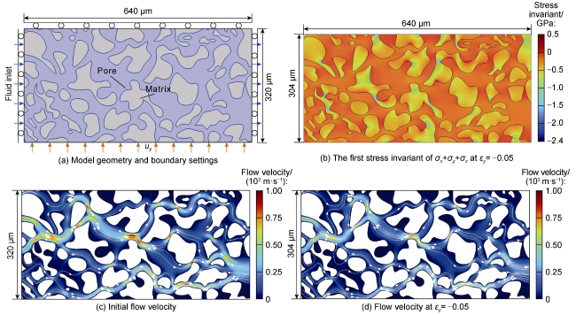
Fig. 4 Model stress and flow velocity distribution when εy=−0.05. |
In the solid mechanics calculation, a specified normal displacement condition was applied to the left (or lower) boundary of the model, while the normal displacement of the remaining boundaries was limited to zero to simulate a specified apparent strain. Two distinct linear elastic materials were adopted within the simulation area to distinguish between the matrix and pores. The matrix area was characterized by an elastic modulus of 27 GPa, a Poisson's ratio of 0.17, and a density of 2 500 kg/m3. In contrast, the pore area was defined with an elastic modulus of 2.16 GPa, a Poisson's ratio of 0, and a density of 1000 kg/m3.
In the calculation of permeability in x direction, the left boundary of the pore area was set as the inlet, with a static pressure of 1 MPa. Meanwhile, the right boundary was designated as the outlet, with a static pressure of 0. The upper and lower boundaries were symmetrical, without considering the influence of gravity. The outlet flow rate was obtained by integrating the outlet flow velocity, and the permeability was calculated using the Darcy's law. For the calculation of permeability in y direction, the lower and upper boundaries of the pore area were set as the inlet and outlet, respectively, with a static pressure of 1 MPa and 0, respectively. Furthermore, the left and right boundaries were maintained as symmetrical. The apparent strains in x and y directions were set as 0, -0.01, -0.02, -0.03, -0.04 and -0.05 to obtain the deformation state of the model under different apparent strains. Subsequently, the mesh after deformation was employed for seepage simulation to calculate permeability in various directions under different strains.
The ADPM and Kozeny-Carman models were applied to fit the changes in simulated permeability (Fig. 5 ). The same set of fitting parameters was used for the permeability in x direction (Fig. 5a, 5b, and 5c ) and y direction (Fig. 5d, 5e, and 5f ), respectively. It was evident that the goodness of fit (R2) of the ADPM model was significantly higher than that of the Kozeny-Carman model, with ADPM models yielding R2 above 0.99. This demonstrates that the anisotropic model presented in this study offers obvious advantages in uniaxial strain, effectively reflecting the varying impacts of compression in different directions on permeability. Furthermore, both ADPM model and Kozeny-Carman model fitted better in case of biaxial uniform compression, indicating that the Kozeny-Carman model is mainly suitable for the isotropic uniform deformation process.
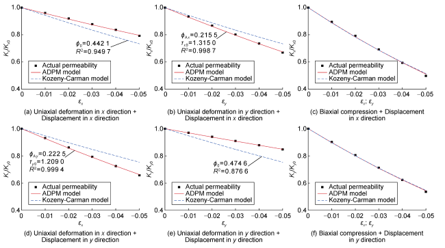
Fig. 5 Permeability changes in different directions at different deformation states. |
5. Model feature analysis
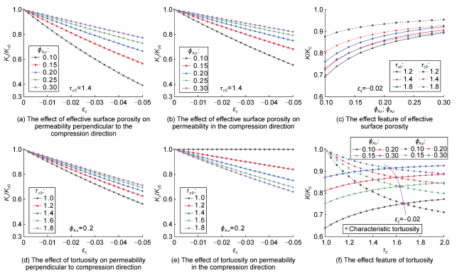
Given that the vertical dimension is significantly smaller than the horizontal dimension in practical scenarios of underground layered oil and gas reservoir development, stress sensitivity analysis is generally simplified as a vertical uniaxial strain process. In this simplified context, the strain in x and y directions is 0, while there is a compressive strain in z direction. Fig. 6 explicates the change characteristics of permeability in each direction during under uniaxial strain in z direction. Fig. 6a and Fig. 6b demonstrate that the effective surface porosity consistently influences permeability in all directions. As the effective surface porosity decreases, permeability becomes more sensitive to strain. Fig. 6 c reveals that when the effective surface porosity remains consistent in all directions, changes in this parameter will not affect the relative relationship of permeability variation magnitude in each direction. Fig. 6d and Fig. 6e illustrate that tortuosity exerted opposite effects on the permeability in the compression direction and the direction perpendicular to it. The sensitivity of the latter to strain diminishes with increasing tortuosity (Fig. 6d ), while the sensitivity of the former to strain increases (Fig. 6e ). When the tortuosity of the compression direction reaches 1, implying the capillary is a straight capillary in the compression direction, compression deformation no longer affects the permeability in that specific direction.
Fig. 6 Effect of different coefficients on permeability in different directions under uniaxial strain. |
The above features are consistent with the deformation principle of the tortuous capillary illustrated in Fig. 3. As the tortuosity increases, the angle α in the figure becomes smaller. At the moment, compression in the seepage direction exerts a growing effect on the capillary radius, while compression perpendicular to the seepage direction has a decreasing effect on it. When the tortuosity reaches 0, signifying a capillary completely parallel to the seepage direction, the capillary radius is solely affected by deformation perpendicular to the seepage direction.
Based on the reverse trend in Fig. 6d and Fig. 6e , impacts of uniaxial strain on permeability in all directions are consistent at a specific combination of tortuosity. Fig. 6f illustrates the distinctive effects of tortuosity on permeability changes in all directions. It suggests that if the tortuosity in all directions is considered consistent as 1.6, there exists a characteristic tortuosity that unifies the effects of uniaxial strain on permeability in all directions. This characteristic tortuosity gradually decreases with the increase of effective surface porosity. Additionally, Fig. 6f highlights that when the tortuosity is less than 1.6, the impact of the vertical uniaxial strain process on horizontal permeability is greater than that on the vertical permeability for the initial isotropic rock.
The reason for the presence of a critical boundary point around a tortuosity of approximately 1.6 can be analyzed based on the model. Eq. (25) indicates that the change in permeability in each direction depends on variations in capillary radius and tortuosity. Based on Eq. (39), Eq. (40) and Eq. (41), the initial tortuosity of $\sqrt{3}$ in each direction reflects the equivalent inclined capillary as the body diagonal of the cube. Under this condition, strain in any direction influenced the radius of the capillary in all directions equally. However, when the initial tortuosity is less than $\sqrt{3}$, the strain in a certain direction exerts a greater effect on the radius of the capillary perpendicular to that direction; in contrast, if it is greater than $\sqrt{3}$, the opposite is true. Eq. (30) further suggests that the strain in a certain direction plays an opposite effect on the tortuosity in that direction and the direction perpendicular to it. Taking compressive strain as an example, compressive strain in a given direction causes a reduction in the total length of the tortuous capillary and the apparent length in the compression direction. Nevertheless, the length of the tortuous capillary in the non-compression direction induces a smaller relative reduction in the total length of the tortuous capillary in comparison to that in the apparent length in the compression direction. Consequently, the tortuosity in the compression direction increases. However, the apparent length perpendicular to the compressed direction remains constant, resulting in a corresponding decrease in tortuosity. These changes are opposite. Considering uniaxial compressive strain of rock with consistent initial tortuosity in all directions (τx0=τz0=τ0) along z direction, if ${{\tau }_{0}}<\sqrt{3}$, then ${{{r}_{x}}}/{{{r}_{x0}}}\;<{{{r}_{z}}}/{{{r}_{z0}}}\;$; if ${{\tau }_{0}}=\sqrt{3}$, then ${{{r}_{x}}}/{{{r}_{x0}}}\;={{{r}_{z}}}/{{{r}_{z0}}}\;$; if ${{\tau }_{0}}>\sqrt{3}$, then ${{{r}_{x}}}/{{{r}_{x0}}}\;>{{{r}_{z}}}/{{{r}_{z0}}}\;$. The tortuosity is always ${{{\tau }_{x0}}}/{{{\tau }_{x}}}\;>1>{{{\tau }_{z0}}}/{{{\tau }_{z}}}\;$. Obviously, only when ${{\tau }_{0}}<\sqrt{3}$, there may be consistent changes in permeability in all directions. According to Fig. 6f , in terms of the porosity range of the conventional rock, the characteristic tortuosity is primarily situated around 1.6 ± 0.05.
In the case of real rock samples, it is generally believed that the tortuosity in the vertical direction tends to be greater than that in the horizontal direction. Consequently, if the tortuosity in horizontal direction is 1.2, only when the tortuosity in vertical direction reaches over 2.0 can a consistent effect of vertical uniaxial strain on permeability in all directions be achieved, as given in Fig. 6f .
6. Conclusions
During the exploitation of layered oil and gas reservoir under uniaxial strain, the impact of effective surface porosity on permeability in all directions is consistent. The sensitivity of permeability to strain increases with decrease of the effective surface porosity. The sensitivity of permeability perpendicular to the compression direction to strain decreases with increasing tortuosity, while that in the compression direction increases.
In the case of layered oil and gas reservoirs with identical initial tortuosity values in all directions, the tortuosity plays a critical role in determining the relative relationship between the amplitude of variation in permeability in all directions during the pore pressure drop. Specifically, when the tortuosity is less than 1.6, there is a more significant decrease in horizontal permeability compared to vertical permeability, while the opposite is true when the tortuosity is greater than 1.6. This distinctive behavior cannot be adequately captured by traditional dynamic permeability models.
The validation of the ADPM through pore-scale simulation experiments demonstrates that the new model exhibits a high fitting accuracy and can effectively characterize the effects of deformation in different directions on the permeability in all directions.
Nomenclature
A—the area of the y-z cross-section of the rock, m2;
D—rock particle diameter, m;
G, Gs—shear modulus of appearance and frame material of the rock (satisfying the elastic constant relationship of isotropic materials), respectively, Pa;
i, j—the dimension of the Cartesian coordinate system, with values of x, y, and z. If they are xx, yy, and zz, they are abbreviated as x, y, and z;
K—permeability, m2;
K0—initial permeability, m2;
Ki, Ki0—current and initial permeability in i direction, respectively, m2;
lx, lx0—current and initial true capillary length of the seepage in x direction, respectively, m;
Lx, Lx0—current and initial apparent length of the rock in x direction, respectively, m;
Mp, Ms—bulk modulus of rock appearance and frame materials, respectively, Pa;
N—number of capillaries per unit area, m−2;
p—pore pressure, Pa;
Δp—increment of current pore pressure compared to the initial, Pa;
q—single capillary flow rate, m3/s;
ri, ri0—current and initial capillary hydraulic radius of the seepage in i direction, respectively, m;
R2—goodness of fit, dimensionless;
ui, uj—displacement of the rock in i and j directions, respectively, m;
V, V0—current and initial apparent volume, respectively, m3;
Vs, Vs0—current and initial frame volume, respectively, m3;
w, w0—current and initial length of the line segment OB in Fig. 3 , respectively, m;
xi, xj—coordinate values of the i and j dimensions, respectively, m;
α, β, γ—∠OBA, ∠HOC and ∠GOC in Fig. 3 , (°);
δij—Kronecker function (if i≠j, δij=0; if i=j, δij=1), dimensionless;
ε, εs—volumetric strain of rock appearance and frame, respectively, dimensionless;
εi, εs,i—normal strain of the rock appearance and frame in i direction, respectively, dimensionless;
εij, εs,ij—components of rock apparent and frame strain, respectively, dimensionless;
εAi, εs,Ai—apparent and frame area strain of the cross-section perpendicular to the capillary seepage in i direction, respectively, dimensionless;
εGH, εOB, εOC, εNM—strain in GH, OB, OC and NM directions of line segments in Fig. 3 , respectively, dimensionless;
μ—fluid viscosity, Pa·s;
$\nu $, ${{\nu }_{\text{s}}}$—Poisson’s ratio of rock appearance and frame materials, respectively, dimensionless;
σs,i—true frame normal stress of the rock in i direction, Pa;
σij, σs,ij, σt,ij—components of rock frame stress, true frame stress, and total stress (positive for tension and negative for compression), respectively, Pa;
τ—capillary tortuosity (ratio of true capillary length to apparent rock length), dimensionless;
τi, τi0—current and initial capillary tortuosity in i direction, respectively, dimensionless;
ϕ, ϕ0—current and initial porosity, respectively, dimensionless;
ϕAi—effective surface porosity of the cross-section perpendicular to the capillary seepage in i direction, dimensionless;
ϕx, ϕx0—current and initial effective porosity of seepage in x direction, respectively, dimensionless.