

Introduction
Enhancing shale gas ultimate recovery is the key task for oil and gas development in China. In the middle and later stages of oil and gas development, affected by scale formation, micro-particle migration and fracture closure, the conductivity of the first fracturing fracture and the permeability of the nearby formation gradually decrease, and the shale gas productivity decreases significantly, making it difficult to produce oil and gas in some areas [1]. In order to avoid reservoir damage and improve ultimate reservoir recovery, refracturing technology has become an important way to tap the potential of remaining shale gas in old wells [2-3].
As early as the 1990s, Elbel et al. [4] proved for the first time through experiments that initial fracturing of oil and gas wells could reverse the principal stress direction by 90°. Subsequently, Wright et al. [5], based on the elastic mechanics of porous media, explained the internal mechanism of stress field changes induced by pore pressure reduction from the perspective of reservoir compaction and fracture slip. Gupta et al. [6] believed that there is a relationship between the change of stress field and reservoir development, and the smaller the initial horizontal principal stress difference of the reservoir, the more conducive to the in-situ stress reversal. Roussel et al.[7] verified the stress reversal phenomenon and concluded that the principal stress direction around the infill well was reversed by 90°. Safari et al. [8-9] found that due to the stress reorientation of horizontal wells, hydraulic fractures may bend or straight fractures may form during the fracturing process of infill wells, mainly depending on the reversal of the principal stress. However, they did not provide a method for optimizing the fracturing timing of infill wells. Sangnimnuan et al. [10] established a coupled seepage-geomechanics model based on an embedded discrete fracture model, which was used to characterize the stress field induced by pressure depletion in unconventional reservoirs with complex geometric fractures. They obtained conclusions similar to those of Gupta. Kumar et al. [11] established a three-dimensional fully coupled model to simulate the stress redirection behavior caused by production, and obtained the fracture propagation trajectory of infill wells affected by stress redirection. Sangnimnuan et al. [12] found that stress reversal has a significant impact on the selection of refracturing methods by studying the pressure and stress distribution after the pressure depletion of fractured reservoirs. Ibáñez et al. [13] developed an integrated multidisciplinary workflow that can screen suitable candidate wells and evaluate the feasibility of refracturing candidate wells using geomechanical modeling. Zhu et al. combined Eclipse and ABAQUS to propose a numerical simulation method for four-dimensional in-situ stress evolution of multiple physical fields in tight sandstone reservoirs during injection and production development [14-15]. Xia et al. [16] established a stress field evolution prediction model, revealing the law of in-situ stress evolution induced by intra and inter layer mining in vertically heterogeneous shale reservoirs. Guo et al. also pointed out that the changes in production-induced stress field are very important for the design of refracturing, but did not provide the optimal timing for refracturing from the perspective of stress evolution [17-18].
There are still some problems such as unclear stress redirection rule and incomplete optimization methods in the timing optimization of refracturing in old wells. Based on the elastic mechanics theory of porous media, embedded discrete fracture model and finite volume method, the seepage-geomechanical coupling model considering the microscopic flow mechanism of shale gas is derived and established in this paper, and the effects of production time, formation permeability and initial formation stress difference on the evolution of stress redirection and the optimal selection of refracturing time are studied using data from shale gas well in Fuling of Sichuan Basin.
1. Optimization of old well refracturing timing
In the early stage, there was insufficient understanding of shale gas reservoir stimulation, shale gas wells faced the problems such as unreasonable fracturing construction scale and displacement and large cluster spacing, and some shale gas wells had fast production capacity depletion and low recovery rate and economic benefits. Therefore, refracturing has become an important measure for tapping the remaining gas potential of old wells.
1.1. Optimization method for the refracturing timing of shale gas wells
According to the different target areas of refracturing, the commonly used refracturing methods are classified into two types. Among them, the fracturing method I refers to extending the original hydraulic fracture without temporarily plugging (Fig. 1a ), and mainly exploiting the remaining gas in the areas beyond the end region of the hydraulic fracture (region A). The refracturing method II is to temporarily plug the old hole and perforate a new one to initiate the new fractures (Fig. 1b ), and mainly excavate the remaining gas inside and near the hydraulic fracture (region B). The degree of stress redirection varies greatly in different regions of the reservoir with different production time, and the fracture trajectories obtained by different refracturing methods are also different. When there is no principal stress reversal at the fracture end and near the wellbore, the fracture generally extends along the red dotted arrow in the figure (perpendicular to the direction of the wellbore) and through the target exploitation area. After the principal stress is reversed at the fracture end and near the wellbore, the fracture generally extends along the yellow dotted arrow (parallel to the maximum horizontal principal stress direction) to converge with the first fracturing fracture. It can be seen that when the principal stress near the fracture end and the wellbore is not reversed or the degree of stress deflection is weak (the angle between the maximum horizontal principal stress and the horizontal wellbore is close to 90°), the refracturing has a higher success rate.
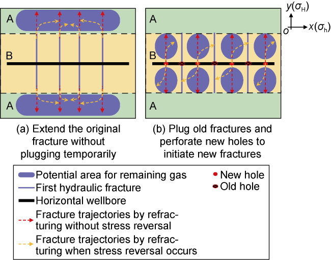
Fig. 1 Schematic diagram of two main refracturing methods of old wells. |
According to the above analysis, the refracturing timing of old shale gas well can be optimized in five steps: (1) Establish a geological model based on reservoir parameters; (2) Inverse fracture parameters using the in-situ fracturing pressure data; (3) Fit reservoir stress evolution with production data; (4) Clarify the relationship between stress reversal area percentage and mining time; (5) Combined with the production situation and development needs of a single well, optimize the refracturing timing comprehensively.
1.2. Seepage-geomechanical coupling model based on pore elasticity theory
The stress balance equation of linearly elastic reservoir can be expressed as [19]:
$\nabla \cdot \sigma +{{\rho }_{\text{r}}}g\text{=0}$
According to Biot theory of porous elastic medium, the pore elastic equation applicable to porous solid medium is as follows [19]:
$\sigma -{{\sigma }_{0}}={{C}_{\text{dr}}}:\varepsilon -b\left( p-{{p}_{0}} \right)I$
$\frac{1}{{{\rho }_{\text{g}}}}\left( m-{{m}_{0}} \right)=b{{\varepsilon }_{\text{v}}}+\frac{1}{M}\left( p-{{p}_{0}} \right)$
where
$b=1-\frac{{{K}_{\text{dr}}}}{{{K}_{\text{s}}}}\ \ \ \ \ \ \ \ \frac{\text{1}}{M}=\phi {{c}_{\text{g}}}+\frac{b-\phi }{{{K}_{\text{s}}}}$
${{K}_{\text{dr}}}\text{=}\frac{E\left( 1-\nu \right)}{\left( 1+\nu \right)\left( 1-2\nu \right)}\ \ \ \ \ \ \ \ \varepsilon \text{=}\frac{\text{1}}{\text{2}}\left[ \nabla u+{{\left( \nabla u \right)}^{\text{T}}} \right]$
A new stress-strain relationship can be obtained by substituting one third of the stress tensor trace (σv=Tr(σ)/3) into Eq. (2):
$\left( {{\sigma }_{\text{v}}}-{{\sigma }_{\text{v,0}}} \right)+b\left( p-{{p}_{0}} \right)\text{=}{{K}_{\text{dr}}}{{\varepsilon }_{\text{v}}}$
By substituting Eqs. (2), (3), (4) into Eq. (1) and ignoring the influence of gravity term, the stress balance equation can be expressed as:
$\nabla \cdot \left[ \mu \nabla u+\mu {{\left( \nabla u \right)}^{\text{T}}}+I\lambda {{T}_{\text{r}}}\left( \nabla u \right) \right]+\nabla \cdot {{\sigma }_{0}}-b\nabla p+b\nabla {{p}_{0}}=0$
Under the small deformation hypothesis, the fluid mass conservation equation is:
$\frac{\partial m}{\partial t}+{{\rho }_{\text{g}}}\nabla \cdot v={{\rho }_{\text{g}}}q$
By substituting Eq. (3) into Eq. (6), the mass conservation equation of formation pressure and strain can be obtained:
$\frac{\text{1}}{M}\frac{\partial p}{\partial t}+b\frac{\partial {{\varepsilon }_{\text{v}}}}{\partial t}+\nabla \cdot v=q$
Considering the influence of shale gas adsorption on porosity, the Biot modulus is modified as follows [20]:
$\frac{\text{1}}{M}=\phi {{c}_{\text{g}}}+\frac{b-\phi }{{{K}_{\text{s}}}}\frac{{{m}_{\text{ad}}}}{{{\rho }_{\text{g}}}}$
Considering various seepage mechanisms of shale gas in matrix pores, the flow velocity v can be expressed as [21]:
$v=-\frac{\prod\limits_{i}{{{F}_{\text{app},i}}}K}{{{\mu }_{\text{g}}}}\nabla p$
The following equation can be obtained by substituting Eqs. (8) and (9) into Eq. (7):
$\left( \phi {{c}_{\text{g}}}+\frac{b-\phi }{{{K}_{\text{s}}}}\frac{{{m}_{\text{ad}}}}{{{\rho }_{\text{g}}}} \right)\frac{\partial p}{\partial t}+b\frac{\partial {{\varepsilon }_{\text{v}}}}{\partial t}+\nabla \cdot \left( -\frac{\prod\limits_{i}{{{F}_{\text{app},i}}}K}{{{\mu }_{\text{g}}}}\nabla p \right)=q$
$\left( \phi {{c}_{\text{g}}}+\frac{b-\phi }{{{K}_{\text{s}}}}\frac{{{m}_{\text{ad}}}}{{{\rho }_{\text{g}}}}+\frac{{{b}^{2}}}{{{K}_{\text{dr}}}} \right)\frac{\partial p}{\partial t}+\frac{{{b}^{2}}}{{{K}_{\text{dr}}}}\frac{\partial {{\sigma }_{\text{v}}}}{\partial t}-$ $\nabla \cdot \left( \frac{\prod\limits_{i}{{{F}_{\text{app},i}}}K}{{{\mu }_{\text{g}}}}\nabla p \right)=q$
Rewrite Eq. (11) in a form including displacement:
$\left( \phi {{c}_{\text{g}}}+\frac{b-\phi }{{{K}_{\text{s}}}}\frac{{{m}_{\text{ad}}}}{{{\rho }_{\text{g}}}}+\frac{{{b}^{2}}}{{{K}_{\text{dr}}}} \right)\frac{\partial {{p}_{n}}}{\partial t}-\frac{{{b}^{2}}}{{{K}_{\text{dr}}}}\frac{\partial {{p}_{n-1}}}{\partial t}+$ $b\frac{\partial \left( \nabla \cdot u \right)}{\partial t}-\nabla \cdot \left( \frac{\prod\limits_{i}{{{F}_{\text{app},i}}}K}{{{\mu }_{\text{g}}}}\nabla {{p}_{n}} \right)=q$
Eqs. (5) and (12) are the main solving equations of the seepage and geomechanics coupled model based on the Biot theory.
1.3. Micro seepage mechanism of shale gas
${{m}_{\text{ad,L}}}={{\rho }_{\text{r}}}{{\rho }_{\text{gsc}}}\frac{p{{V}_{\text{L}}}}{p+{{p}_{\text{L}}}}$
${{m}_{\text{ad,B}}}={{\rho }_{\text{r}}}{{\rho }_{\text{gsc}}}\frac{{{V}_{\text{m}}}C{{p}_{\text{r}}}}{1-{{p}_{\text{r}}}}\left[ \frac{1-\left( d+1 \right)p_{\text{r}}^{d}+dp_{\text{r}}^{d\text{+1}}}{1+\left( C-1 \right){{p}_{\text{r}}}-Cp_{\text{r}}^{d\text{+1}}} \right]$
where
${{p}_{\text{r}}}=\frac{p}{{{p}_{\text{s}}}}\ \ \text{ }\ {{p}_{\text{s}}}=\exp \left( 7.743\ 7-\frac{1\ 306.548\ 5}{19.436\ 2+{{T}_{\text{m}}}} \right)$
${{F}_{\text{app}}}=\left( 1+\beta \text{ }Kn \right)\left( 1+\frac{4Kn}{1+Kn} \right)$
where
$Kn=\frac{{{\mu }_{\text{g}}}}{2.828\ 4p}\sqrt{\frac{\pi R{{T}_{\text{m}}}}{2{{M}_{\text{g}}}}\frac{\phi }{K}}\ \ \ \beta =\frac{128}{15{{\pi }^{2}}}{{\tan }^{-1}}\left( 4K{{n}^{0.4}} \right)$
1.4. Fully coupled model of seepage and geomechanics
The core idea of the embedded discrete fracture model is to use structured grids to independently establish the simulation domain corresponding to the matrix and fracture, and describe the flow relationship between matrix and fracture through non-adjacent conductivity [26]. For any fracture unit and its corresponding matrix unit, the volumetric flow rate between the two can be expressed as:
${{q}_{\text{f-m}}}={{\lambda }_{\text{t}}}{{T}_{\text{f-m}}}\Delta p$
The conductivity is mainly influenced by the permeability and geometric shape of the matrix and fracture segments, resulting in [27]:
${{T}_{\text{f-m}}}=\frac{2{{A}_{\text{f}}}\left( K\cdot n \right)\cdot n}{{{d}_{\text{f-m}}}}$
For two intersecting fractures, the conductivity between intersecting fracture units can be expressed as [28]:
${{T}_{\text{f-f}}}=\frac{{{T}_{1}}{{T}_{2}}}{{{T}_{1}}+{{T}_{2}}}$
By substituting the flow exchange term Eq. (16) between matrix and fracture into Eq. (12), the flow equation within the matrix considering the influence of the fracture system can be obtained:
$\left( \phi {{c}_{\text{g}}}+\frac{b-\phi }{{{K}_{\text{s}}}}\frac{{{m}_{\text{ad}}}}{{{\rho }_{\text{g}}}}+\frac{{{b}^{2}}}{{{K}_{\text{dr}}}} \right)\frac{\partial {{p}_{n}}}{\partial t}-\frac{{{b}^{2}}}{{{K}_{\text{dr}}}}\frac{\partial {{p}_{n-1}}}{\partial t}+b\frac{\partial \left( \nabla \cdot u \right)}{\partial t}-$ $\nabla \cdot \left( \frac{\prod\limits_{i}{{{F}_{\text{app},i}}}K}{{{\mu }_{\text{g}}}}\nabla {{p}^{n}} \right)+\frac{{{\lambda }_{\text{t}}}{{T}_{\text{f-m}}}\left( p_{\text{f,}n}^{{}}-{{p}_{n}} \right)}{{{V}_{\text{c}}}}=q$
Similarly, the flow equation within the fracture can be obtained:
$\left( \frac{1}{{{M}_{\text{f}}}}+\frac{{{b}^{2}}}{{{K}_{\text{dr}}}} \right)\frac{\partial p_{\text{f,}n}^{{}}}{\partial t}-\frac{{{b}^{2}}}{{{K}_{\text{dr}}}}\frac{\partial p_{\text{f,}n\text{-1}}^{{}}}{\partial t}-\nabla \cdot \left( \frac{{{K}_{\text{f}}}}{{{\mu }_{\text{g}}}}\nabla p_{\text{f,}n}^{{}} \right)+$ $\frac{{{\lambda }_{\text{t}}}{{T}_{\text{f-m}}}\left( {{p}_{n}}-p_{\text{f,}n}^{{}} \right)}{{{V}_{\text{c}}}}+\frac{{{\lambda }_{\text{t}}}{{T}_{\text{f-f}}}\left( p_{\text{f}1,n}^{{}}-p_{\text{f}2,n}^{{}} \right)}{{{V}_{\text{c}}}}=q$
By combining Eqs. (2), (3), (5), (19) and (20), the stress along the y-axis direction σyy, the stress along the x-axis direction σxx and the induced shear stress σxy can be obtained. According to the following equations, the maximum and the minimum horizontal principal stresses (σH and σh) and the azimuth angle α can be calculated:
$\left\{ \begin{align} & {{\sigma }_{\text{H}}}=\frac{{{\sigma }_{xx}}+{{\sigma }_{yy}}}{2}+\sqrt{{{\left( \frac{{{\sigma }_{xx}}-{{\sigma }_{yy}}}{2} \right)}^{2}}+\sigma _{xy}^{2}} \\ & {{\sigma }_{\text{h}}}=\frac{{{\sigma }_{xx}}+{{\sigma }_{yy}}}{2}-\sqrt{{{\left( \frac{{{\sigma }_{xx}}-{{\sigma }_{yy}}}{2} \right)}^{2}}+\sigma _{xy}^{2}} \\ \end{align} \right.$
$\tan \alpha =\frac{{{\sigma }_{\text{H}}}-{{\sigma }_{xx}}}{{{\sigma }_{xy}}}$
1.5. Model solution
Eqs. (5), (19) and (20) are the main solving equations. After discretizing the above three equations, two coefficient matrix equations containing four unknown variables (ux, uy, p, pf) can be obtained. The iterative method is used to solve the equations according to the calculation process shown in Fig. 2 .
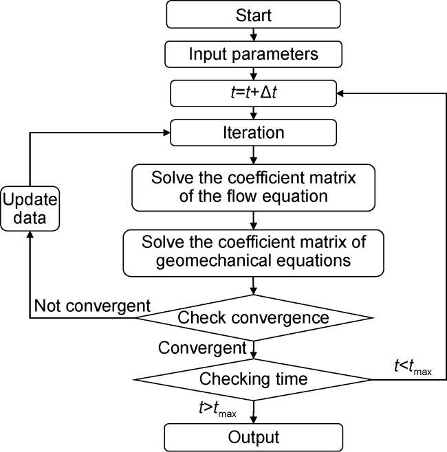
Fig. 2 Model solving process. |
2. Model verification
To verify the accuracy of the proposed model, two models with 50° dip angle and two clusters of fractures were established using structured and unstructured grids respectively, by virtue of the proposed model and COMSOL commercial software. The dimension of both models is 200 m×200 m×20 m. The input parameters are shown in Table 1 . The normal displacement on the boundary was set to 0 for simulation, and the stress distribution along the x-axis after 5 years of production was obtained (Fig. 3 ). It can be seen from the comparison that, affected by the reduction of formation pressure, σxx simulated by the two methods decreases to a large extent near the fracture, but increases significantly in the area far from the end of fracture, and the stress distribution is very close, which proves that the stress calculation accuracy of the model in this paper is high.
Table 1 Main input parameters for model validation |
| Parameter | Value | Parameter | Value |
|---|---|---|---|
| Initial formation pressure | 38 MPa | Fracture half-length | 100 m |
| Langmuir pressure | 4 MPa | Matrix permeability | 300×10−9 μm2 |
| Formation temperature | 343.15 K | Fracture permeability | 2 μm2 |
| Langmuir volume | 0.018 m3/kg | Fracture width | 1×10⁻³ m |
| Matrix porosity | 6% | Bottom hole pressure | 18 MPa |
| Matrix compressibility coefficient | 1.0×10⁻³ MPa−1 | Time | 5 years |
| Fracture porosity | 100% | Stress along the x-axis | 52 MPa |
| Elastic modulus | 29 GPa | Stress along the y-axis | 55 MPa |
| Poisson's ratio | 0.13 | Stress along the z-axis | 56 MPa |
| Biot constant | 0.8 |
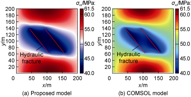
Fig. 3 Comparison of stress distributions along the x-axis simulated by the two methods. |
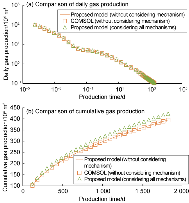
Fig. 4 Comparison of daily gas production and cumulative production calculated by the two methods (the mechanisms refer to microscopic seepage mechanisms of adsorption, desorption, diffusion and slip). |
3. Application case
3.1. Optimal refracturing timing
The horizontal well W1 in the Fuling Shale Gas Field of the Sichuan Basin, SW China, has a continuous reservoir thickness of 38 m in the Longmaxi Formation of Silurian, with an average vertical depth of 2 400 m, a pressure gradient of 1.2 MPa/100 m, a horizontal section length of 1 600 m and a well spacing of 400 m. The fracturing design shows that the well has an average porosity of 4.8%, an average permeability of 0.035×10⁻⁶ μm2, an average Poisson’s ratio of 0.18, an average elastic modulus of 41 GPa, an initial minimum horizontal principal stress of 52 MPa, and an initial stress difference of 5 MPa. According to the design, the 6th fracturing stage is 120 m long and has 3 clusters of fractures. Due to the difficulty of sand addition, the spacing of clusters is designed to be 40 m to reduce stress interference. The designed construction displacement is 14 m3/min, and the total fracturing fluid volume is 1 600 m3. The average effective fracture half-length in this fracturing section is 118 m and the average fracture conductivity is 15 μm2·cm by fitting the field fracturing construction curve of the 6th stage (Fig. 5 ) by means of Meyer fracturing design software. After 3 years of production, the production capacity of Well W1 has decreased to a large extent. In order to further improve its development effect, refracturing is planned. A 400 m×160 m×38 m physical model of shale gas production is established according to geomechanical parameters and fracture parameters.
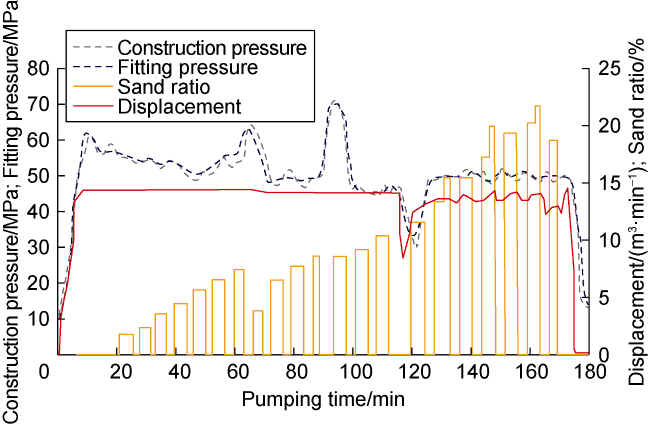
Fig. 5 Fracturing construction curve and fitting curve of the 6th stage of W1 horizontal well. |
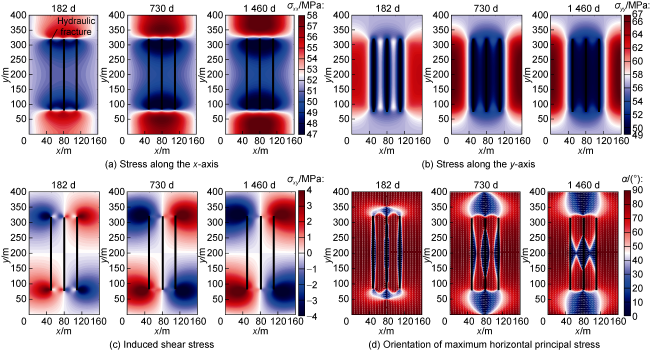
Fig. 6 Distribution of stress and maximum horizontal principal stress orientations at different production times. |
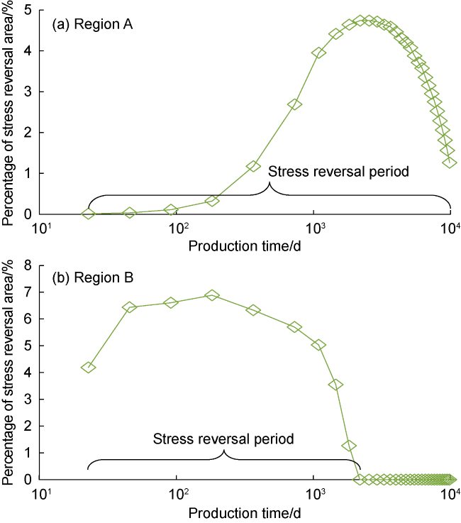
Fig. 7 Relation between the percentage of stress reversal area and production time. |
Considering that Well W1 had already experienced a significant reduction in production rate after 3 years of production, it is clear that implementing refracturing after production of 2 000 or 10 000 d does not meet the economic requirements. Considering the optimal refracturing time and the actual situation on site, it was decided to take the measures such as shut-in or fluid injection to restore formation pressure, so that the internal stress in target regions A and B can be restored to the initial state and the fracture trajectory reaches the ideal position. Well W1 was shut in after 1 255 d of production. After approximately 30 d of shut-in, Well W1 was refractured using method II. Microseismic monitoring of refracturing (Fig. 8 ) shows that the signal points of micro-seismic events of the refracturing are mainly concentrated between the fractures of the primary fracturing, indicating that the new fractures formed by refracturing do not intersect with the old fractures and cross the target residual gas area, which proves that the refracturing stimulation is successful.
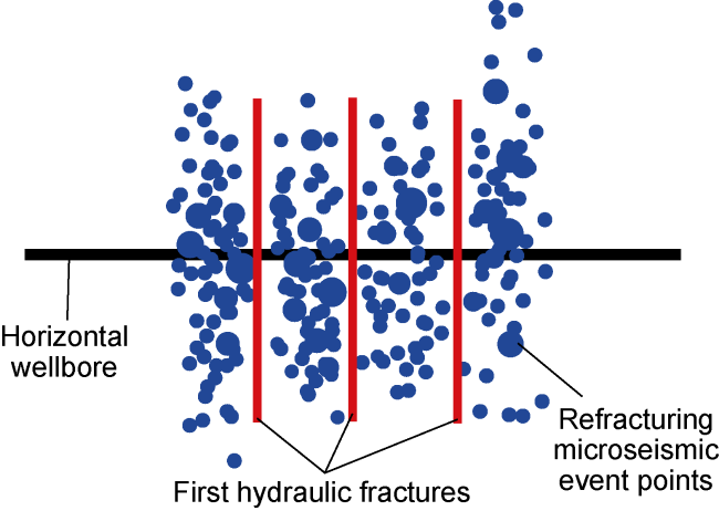
Fig. 8 Microseismic monitoring of refracturing in stage 6 of Well W1 (the size of blue dot represents the intensity of refracturing microseismic event). |
3.2. Factors affecting refracturing timing
3.2.1. Effect of permeability
Using the model of Well W1, the relationship curve between production time and the percentage of stress reversal area in regions A and B was simulated at the set matrix permeability of 0.01×10⁻⁶, 0.10×10⁻⁶, 0.50×10⁻⁶, 1.00×10⁻⁶ μm2 (Fig. 9 ). It can be seen that, (1) the percentage of stress reversal area in region A exhibits different trends with increasing production time due to different matrix permeability. When the matrix permeability is greater than 0.01×10⁻⁶ μm2, the curve first rises and then decreases. When the matrix permeability is equal to 0.01×10⁻⁶ μm2, the curve rises monotonically. Analysis shows that when the matrix permeability is as low as 0.01×10⁻⁶ μm2, shale gas flow is difficult and lasts for a long time, so the data within the simulation time range is not sufficient to reflect the entire process of stress reversal in region A. (2) However, the curve of region B generally shows a trend of rising first and then decreasing under different matrix permeability. This is mainly because region B is generally close to artificial fractures, with a shorter flow distance of shale gas, a faster decrease in formation pressure, and a faster change in stress. On the one hand, the simulation time can reflect the whole process of stress reversal in region B, and on the other hand, it can be seen that the peak of the curve under the same matrix permeability condition appears earlier in region B than in region A. (3) With the increase of matrix permeability, the peak of curve in region A and region B appear earlier, and the stress reversal disappears earlier as well, so refracturing measures should be taken earlier. (4) When the matrix permeability ranges from 0.1×10⁻⁶ μm2 to 1.0×10⁻⁶ μm2, the optimal time for refracturing method I in region A is 1 460−10 000 d, and the optimal time for refracturing method II in region B is 182−2 190 d. (5) When the matrix permeability decreases to 0.01×10⁻⁶ μm2, the theoretically optimal time for refracturing will far exceed 10 000 d. Under this condition, the production capacity of a single well will decrease rapidly. To ensure economic efficiency, measures such as well shut-in or gas injection can be taken to restore stress and refracturing can be implemented in advance.
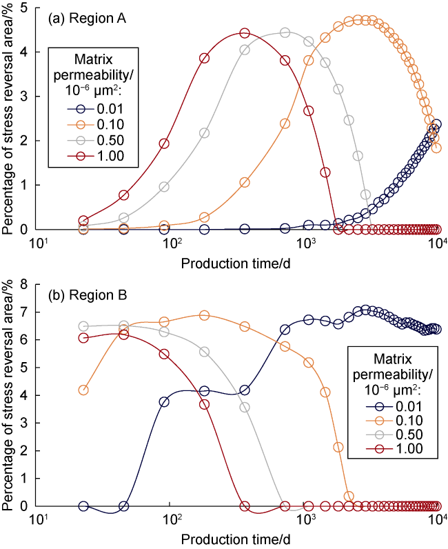
Fig. 9 Influence of matrix permeability on the stress reversal area percentage. |
3.2.2. Effect of initial stress difference
The model of Well W1 was adopted, and the initial stress difference was set at 3, 5, 7, and 9 MPa to simulate the relationship between production time and the percentage of stress reversal area (Fig. 10 ). As can be seen from the figure, (1) The larger the initial stress difference is, the shorter the time required for the stress reversal area percentage curve return to zero (return to the initial state) after rising first and then declining, and the earlier the optimum time to carry out refracturing. (2) Because region B is close to the artificial fractures, the peak and zero value of its curve appear earlier than those of region A under the same initial stress difference condition. (3) When the initial stress difference is 3-7 MPa, the optimal time of refracturing method I in region A needs to be greater than 6 570 d, and when the initial stress difference reaches 9 MPa, the curve remains on 0 continuously, and no stress reversal occurs, so refracturing can be implemented at any time. (4) For the potential gas tapping area in region B, the optimal time of refracturing method II is 730-3 650 d. (5) Under the same matrix permeability and initial stress difference, the optimal time of refracturing method I is later than that of method II, excluding the interference of human factors.
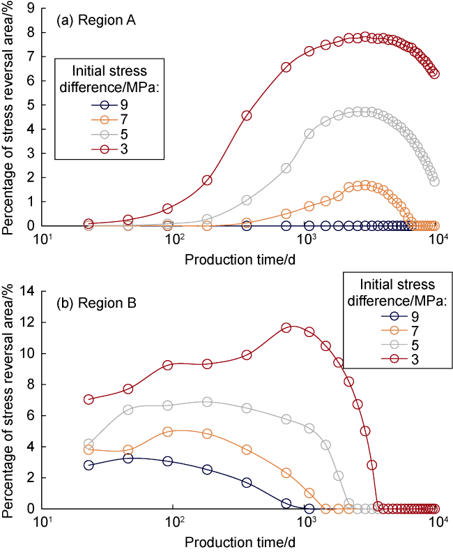
Fig. 10 Influence of initial stress difference on the stress reversal area percentage. |
3.2.3. Effect of natural fracture distribution
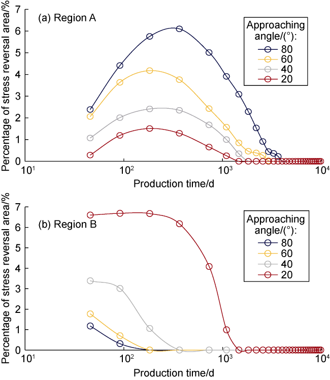
Based on the model of Well W1, 400 natural fractures with a length of 30 m and permeability of 0.01 μm2 were randomly generated, and the approaching angles of natural fractures were set as 80°, 60°, 40°, and 20° to simulate the influence of different fracture approaching angles on the orientation distribution of the maximum horizontal principal stress (Fig. 11 ). The relationship curve between production time and percentage of stress reversal area was obtained (Fig. 12 ). The comparative analysis shows that, (1) the larger the natural fracture approaching angle, the more difficult it is to have stress reversal in region B, and the earlier the optimum time to carry out refracturing. (2) The more easily the stress reversal occurs in region A, the later the optimum time to start refracturing. The optimal time to implement refracturing method I in region A is 1 825-3 650 d. The optimum time to implement refracturing method II in region B is 152-1 460 d.

Fig. 11 Influence of fracture approaching angle on orientation distribution of maximum horizontal principal stress. |
Fig. 12 Effect of natural fracture approaching angle on percentage of stress reversal area. |
4. Conclusions
Under the influence of formation pressure depletion, the percentage of stress reversal area near the fracturing well first increases and then decreases with the extension of time, and the closer the area is to the artificial fracture, the shorter the peak time of the stress reversal area percentage curve, and the shorter the time for the final return to zero (return to the initial state).
The optimum time of refracturing shale gas well is affected by matrix permeability, initial stress difference and natural fracture approaching angle. The larger the matrix permeability and the initial stress difference are, the shorter time it takes for stress reversal area percentage curve to reach the peak and return to the initial state, and the earlier refracturing measures shall be taken. The larger the natural fracture approaching angle is, the more difficult the stress reversal is to occur near the fracture, and the earlier the optimal time of refracturing is, while the easier the stress reversal is to occur in the parts far from the fracture end, and the later the optimal time of refracturing is.
In the shale gas reservoir with ultra-low matrix permeability, the productivity of a single well decreases quickly. In order to ensure economy, measures such as well shut-in or gas injection for energy recovery can be taken to restore stress and refracturing can be implemented in advance.
Nomenclature
Af—the intersection area between the matrix unit and the fracture unit, m2;
b—Biot coefficient, dimensionless;
cg—compressibility coefficient of shale gas, Pa−1;
C—BET adsorption constant, dimensionless;
Cdr—fourth-order elastic tensor, Pa;
d—number of BET adsorbed molecular layers;
df-m—the mean normal distance from matrix unit to fracture plane, m;
E—elastic modulus of rock, Pa;
Fapp—correction factor for shale gas permeability, dimensionless;
g—acceleration of gravity, m/s2;
I—unit tensor, dimensionless;
K—matrix permeability tensor, m2;
K—matrix permeability, m2;
Kf—fracture permeability tensor, m2;
Kdr—volume modulus of dry rock, Pa;
Ks—volume modulus of rock, Pa;
Kn—Knudsen number, dimensionless;
m—fluid mass per unit rock volume, kg/m3;
mad—adsorbed gas per unit matrix volume, kg/m3;
mad,L, mad,B—adsorbed gas volume based on single-layer Langmuir isotherm and multi-layer BET isotherm, kg/m3;
M—Biot modulus, Pa;
Mf—Biot modulus in fracture simulation domain, Pa;
Mg—molecular weight of shale gas, kg/mole;
n—time step;
n—normal vector of fracture surface, dimensionless;
p—fluid pressure, Pa;
pf, pf1, pf2—fluid pressure in fracture, fracture 1 and fracture 2, Pa;
pr—intermediate variable, dimensionless;
ps—pseudo-saturation pressure, Pa;
pL—Langmuir pressure, Pa;
Δp—pressure difference between matrix unit and fracture unit, Pa;
q—fluid source sink term, s−1;
qf-m—the flow rate between the fracture unit and the corresponding matrix unit, m3/s;
R—Boltzmann constant, J/(K·mol);
t—time, s;
tmax—the maximum time of simulation, s;
Δt—the length of the time step, s;
Tm—reservoir temperature, K;
T1, T2—conductivity of fracture unit 1 and fracture unit 2, m3;
Tf-f—conductivity between intersecting fracture units, m3;
Tf-m—conductivity between the fracture unit and the matrix unit, m3;
Tr—trace of a matrix (sum of all elements on the main diagonal of matrix);
u—displacement vector, m;
ux, uy—displacement along the x and y axes, m;
v—flow velocity, m/s;
Vc—matrix unit volume, m3;
VL—Langmuir volume, m3/kg;
Vm—BET adsorption volume, m3/kg;
α—the angle between the maximum horizontal principal stress and the x-axis (the orientation of the maximum horizontal principal stress), the one in the initial state is 90°, (°);
β—sparse parameter, dimensionless;
ε—second-order strain tensor, dimensionless;
εv—volumetric strain, dimensionless;
λt—relative mobility, (Pa·s)−1;
λ, μ—the first and the second Lamay constant, Pa;
μg—viscosity of shale gas, Pa•s;
$\nu$—Poisson's ratio, dimensionless;
ρg—shale gas density, kg/m3;
ρgsc—adsorbed gas density, kg/m3;
ρr—rock density, kg/m3;
σ—total stress tensor, Pa;
σh, σH—minimum and maximum horizontal principal stress, Pa;
σxx, σyy, σxy—stress along x axis, stress along y axis and shear-induced stress, Pa;
σv—one-third of the trace of the stress tensor trace σ, Pa;
ϕ—shale porosity, %;
Subscript:
0—initial reference state;
i —matrix unit number.