

Introduction
Depth matching of well logs is a very important data processing task, providing the foundation for accurately acquiring stratigraphic interpretation parameters and conducting reservoir evaluation and analysis, which is crucial for ensuring the accuracy of subsequent geological modeling [1]. During logging operation, there are many factors that affect the depth alignment of sampling points between different well logs. For example, the stretch or contraction of elastic cable may result in significant errors between measurement and actual depth [2]; the reference depths for different logging channels are often not synchronized [3⇓-5]; and well logs may be affected by system noise and downhole environment, leading to depth discrepancies [6]. Almost all well log data should be treated by depth matching before analyzing the lithology and fluid properties of reservoirs; otherwise, logging interpretation would be inaccurate.
In response to these challenges, the researchers in the 1980s proposed various methods which can be summarized into two major categories: depth matching based on statistical methods [7] and feature points alignment based on reference well logs [8]. These traditional methods use the natural gamma ray (GR) logging curves as a reference to align depth points by identifying the sequences with the same geological structural features on different well logging curves. In the 1990s, various commercial software programs were developed and applied, which primarily use the correlation between two signal sequences to make similarity matching [9-10]. However, most of the traditional methods manually pick similar signal sequences on well logs based on subjective human experience [11]. In the early 21st century, Aach et al. [12], Petitjean et al. [13] and Mei et al. [14] introduced a dynamic time warping method (DTW) based on traditional methods to measure the similarity of different signal sequences. However, DTW, as a time series-based local comparison method, is susceptible to data noise and computationally intensive [15-16].
In recent years, with the development of logging technology, thin oil layer interpretation, perforation and logging while drilling (LWD) have all demanded higher efficiency and accuracy of depth matching. Many scholars have attempted to solve the issues using machine learning [17⇓⇓-20], such as fully connected neural network (FCNN) [1], convolutional neural network (CNN) [11,21], and long short-term memory network (LSTM) [22] being proposed and applied to depth matching between gamma ray (GR) logs. However, these methods are only effective for depth matching between GR logs and less effective. Torres et al. [6] proposed the use of one-dimensional CNN to capture the similar features between different well logs, which not only reduces the workload for manually extracting features from well logs but also effectively matches between different types of well logs. However, deep learning requires a large dataset for model training to avoid overfitting [23]. In addition, manual labeling is a cumbersome process. To the end, reinforcement learning was introduced into depth matching [24]. The deep Q-learning network algorithm (DQN) does not require manual labeling but relies on the feedback of a reward signal through the interaction between the agent and the environment to guide the agent to gradually learn the optimal depth matching strategy [8]. However, this single agent reinforcement learning method is limited to depth matching between GR well logs of the same well. This paper further develops a novel depth matching method based on deep reinforcement learning to imitate manual operation to perform depth matching between well logs from multiple wells to improve the efficiency of well log data preprocessing. The method is further improved based on single agent reinforcement learning, adding a scaling mechanism for logging feature sequences in a high dimensional action space, and regarding the depth matching of multiple well logs as a Markov decision process, thereby establishing a multi-agent reinforcement learning prediction system. Field applications have demonstrated the system can significantly improve the efficiency and accuracy of depth matching on conventional well log datasets, achieving the goal of automatic depth matching for multiple wells.
1. Depth matching of well logs
Considering the radioactive sources and safety protection measures, the field logging operations are usually divided into 2 to 3 stages. As shown in Fig. 1 , the first stage involves testing non-radioactive well logs such as natural gamma ray (GR1), spontaneous potential (SP), acoustic time difference (Δt), shallow lateral resistivity (RLLS) and deep lateral resistivity (RLLD). The second stage often includes a GR2 curve and well logs with radioactive sources, like compensated neutron porosity (ϕCNL) and density (ρ) [20]. Due to the complexity of measurement methods and environment, there are often discrepancies between the measured and actual depths of various well logs. According to the discrepancies, depth matching can be categorized into two types.
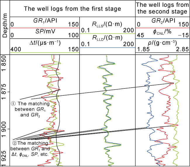
Fig. 1. An example of well log depth matching. |
1.1. Depth matching between GR well logs
During logging operations in the same well in different stages, variations in cable tension occur due to factors such as the lifting speed of the logging tool, the position movement of the derrick pulley, the weight of the logging tool, the friction between the cable and tool string with the wellbore, and drilling mud specific gravity, etc. These variations cause depth discrepancies between different well logs. Whether they are direct or indirect factors, depth errors are inevitable. Consequently, logging companies around the world set the depth delay of the sample points on the well logs recorded in the second stage (ϕCNL, ρ, GR2) as the same as preset values [25]. They use GR1 as a depth reference, and match GR2 with GR1 to make preliminary depth matching of the well logs at different stages (Fig. 1 ).
1.2. Depth matching between different well logs
During the same stage of logging operations, depth discrepancy may arise between different well logs if logging tools are stuck or subjected to runout when lifted up, resulting in the stretch or compression of the well logs. In addition, depth delay of sample points, the friction between logging tools and the wellbore and the adhesion effect of drilling mud may cause depth discrepancy, too. Although the depth errors between well logs measured in the same stage tend to be smaller than those between different stages, they cannot be neglected when downhole conditions are poor. As shown in Fig. 1 , both the depths of Δt, SP and GR1 recorded in the first stage, and the depths of ϕCNL, ρ, etc., recorded in the second stage need to be corrected by referring to GR1.
2. Principle of well log depth matching
2.1. Markov decision process for depth matching of multiple well logs
Reinforcement learning (RL) is a significant branch of machine learning, where the problems that RL aims to solve are typically abstracted into the interactions between the agent and its environment. In this paper, the decision-making subject that learns and implements depth matching of well logs is referred as the agent, and any external entities interacting with the agent are termed the environment, which includes input well logs and historical matching records. The matching status of the current well log observed by the agent in the environment is called a state, and a set of operations (translating, scaling or stopping) taken by the agent to act on the environment to change the matching status of the well log is called an action. RL attempts to solve a Markov decision-making optimization problem based on the interaction between the agent and the environment [26]. In a single-agent system for depth matching, the system can process inputs from two well logs, generally GR1 and GR2 (Fig. 2a ). To achieve simultaneous and automatic depth matching between target well logs (e.g. GR2, ϕCNL, ρ, Δt, etc.) and the reference well log (GR1), this paper defines the execution subject for depth matching of each pair of well logs as an agent. This approach expands the single-agent reinforcement learning system into a multi-agent one (MARL, Fig. 2b ).
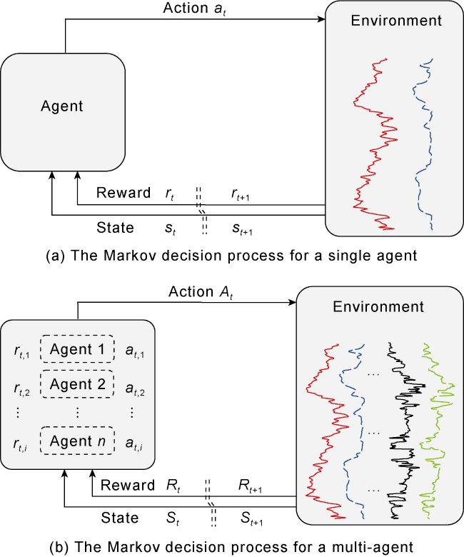
Fig. 2. Schematic diagram of the interaction between the agent and the environment in reinforcement learning. |
Similar to the single-agent reinforcement learning process, the multi-well log depth matching process in a multi-agent system is also a Markov decision process (MDP), as shown in Fig. 2b . The difference is that when multiple agents interact with the same environment, they not only cooperate to observe the environment to update the status and obtain the maximum cumulative reward but also independently complete the depth matching between the corresponding target well log and the reference well log. The interaction process between agents is shown in Fig. 2b . At time t, the ith agent observes the current state of the environment and selects an action under a specific strategy to act on the environment. Then, all agents execute a joint action based on a joint strategy [27]. The environment responds to this action, leading to a new state , and each agent receives a reward . This process is repeated at the next time step t+1, generating a series of rewards and new states , thus creating a Markov decision sequence . Through this iterative cycle, the agents learn an optimal strategy to perform actions and obtain maximize rewards, ultimately achieving automatic matching of multiple well logs.
2.2. Design of the DDQN algorithm for depth matching of multiple well logs
In 2001, Aach et al. [12] introduced a dynamic time warping (DTW) method for aligning different time series of biological gene expressions to observe and analyze the changes in gene activity over time. Subsequently, Wang et al. [11] applied this method for automatic depth matching between the sequences (X={x1, x2,…, xn}) on GR1 and the sequences (Y={y1, y2,…, yn}) on GR2. By constructing a cost matrix ( ) from the Euclidean distances between corresponding points on the well logs, the similarity and matching effect between the sequences are maximized when the cumulative distance between corresponding points in the two sequences is minimized, as shown in Eq. (1). However, when processing well logs with large-scale sampling points, DTW will increase the computational complexity and make the matching results unstable [1]. In response to the above problems, Bittar et al. [24] introduced the DQN method [26] for automatic depth matching between GR logs. This method can quickly and continuously self-learn to improve the control optimization process in the depth matching task. However, DQN faces a significant challenge: when estimating the expected return (Q-value function, as shown in Eq. (2)) for an action ( ) taken by an agent in the current state ( ), the value function update tends to overestimate the Q-values, leading to instability in the training process and ultimately resulting in suboptimal strategy [28]. To address this issue, our study proposes a multi-agent reinforcement learning model based on DDQN, which mitigates overestimation through a dual-network (evaluation and target networks) evaluation mechanism. The DDQN framework for depth matching of multi-well logs (Fig. 3 ) includes a dual sliding window, a dual-network evaluation mechanism and an experience replay pool.
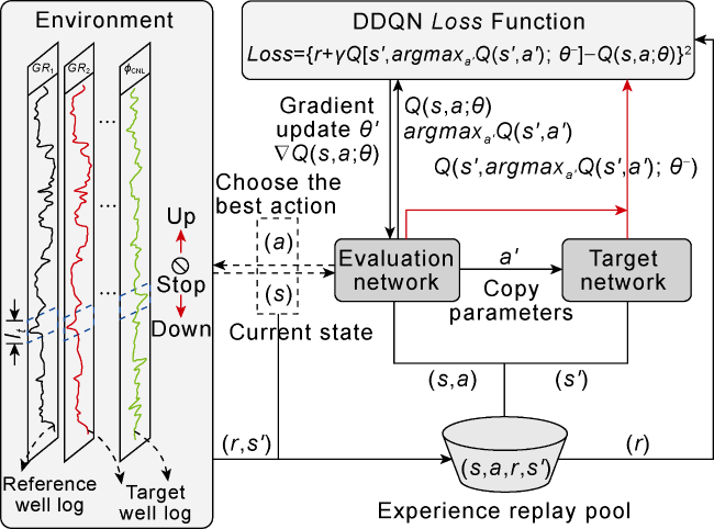
The depth matching task is to convolve the feature sequences on multiple well logs through multiple dual- channel one-dimensional CNN (dual sliding windows) and input them into the DDQN network. One agent can input the feature sequences of two well logs through one dual sliding window. The first sliding window (Win1) moves top-down on the reference well log (GR1), while the second sliding window (Win2) moves up and down on the target well log (GR2, ρ, ϕCNL, etc.) based on the signal sequence within Win1, to extract target sequences with similar features to the reference well log. In the DDQN algorithm architecture shown in Fig. 3 , the center point of the sliding window represents its current depth position on the well log. The first sliding channel of the dual sliding window contains a feature sequence of length (l) on the reference well log, with the window size covering 128 sampling points at a sample interval of 0.125 m; the other channel covers a sequence of the same length on the target well log. Given that a fixed-size sliding window may not easily capture smaller or larger feature sequence segments due to its constant size, this study introduces a variable sliding window. An agent can select a random size through trial and error to find the appropriate feature capture window, as defined in Eqs. (3) and (4). To visually represent the sliding window channels, a segment is cut from the well log (see the red box in Fig. 4 ), with the size of the first sliding window defined in Eq. (3) as Win1. The initial position of the center point of the second sliding window (Win2) is the same as Win1, with the window boundary size randomly generated by the agent. During the top-down sliding matching process, Win2, as defined in Eq. (4), can identify the best matching features on the target well log.
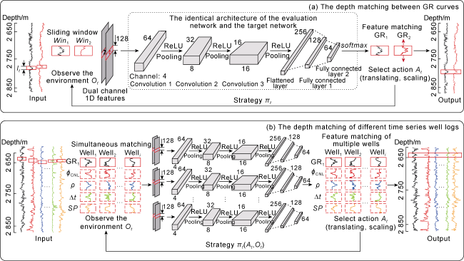
Fig. 4. DDQN network structure for depth matching of multiple well logs. |
Subsequently, the multi-agent system emulates humans to perform depth matching of multiple well logs based on the sequential decision-making process. This process divides each time step t into two steps. The first step is mainly to complete the matching task between the GR well logs measured at different stages within the same well. That is, first set the depth delay of the sampling points on the well logs (GR2, ρ, ϕCNL, etc.) recorded in the second stage in the same well as the same as preset value, ensuring that the depth of the well logs in the second stage is roughly consistent [25]. Then, while matching GR2 with the reference well log GR1, preliminary depth matching is also conducted between well logs ϕCNL, ρ, etc., and GR1. The second step is mainly to fine-tune the depth deviation between the target well logs and GR1 when the depth discrepancies between different types of well logs within the same well cannot be overlooked.
In this way, in the multi-agent depth matching task, each agent at time t obtains a depth matching state by observing the feature sequences of well logs through the dual sliding windows. The first type of agent responsible for the depth matching between GR well logs makes decisions in a predefined order, that is to choose an action ( ) based on the ε-greedy strategy [26] to act on the environment. Subsequently, the second type of agent, responsible for depth matching between the well logs ϕCNL, ρ, Δt, etc., and GR1, selects an action based on the decision-making result of the first type of agent to act on the well log to be matched. At time t, each agent can update to the next state (s') and receive a feedback reward (r) after interacting with the environment. Then the experience replay pool (Dt) collects and stores the experience samples of agents at each time t. As shown in Fig. 3 , during the model training process, DDQN randomly selects a batch of sample data from Dt. It calculates the Q-value Q(s,a;θ) for the selected action (a) in the current state through the evaluation network, and estimates the Q-value of selected action (a') in the next state through the target network. This dual-network structure has the same architecture, and includes three convolutional layers (Fig. 4 ), with each convolutional layer followed by a nonlinear activation function (ReLU) and a max-pooling layer, and the features are integrated through a fully connected layer to output the Q-values. Then, the difference between the Q-values of the evaluation network and the target network under the current strategy is calculated through a loss function (Eq. (5)). By minimizing the loss function, it is used to guide the optimization of the neural network, thereby learning a better matching strategy. Finally, the current evaluation network parameter (θ) is updated to θ' through a stochastic gradient descent (Eq. (6)) for the next round of training and learning. By repeating the above process, each agent can learn how to take the optimal action to complete depth matching for multiple well logs.
2.3. Definition of model attributes
2.3.1. Action space
Action is an important aspect of DDQN, which lists various ways in which an agent interacts with the environment. In this paper, action At=(upgliding, sliding, stop) is defined as a multi-dimensional parameter space where each dimension corresponds to a different type of action, including translating, scaling and stopping. The translating action ( ) is defined as the agent selecting a step size to move the feature sequence up or down on the well log, with the step size ranging from 1 to 40 sample interval units, . The scaling action ( ) mainly involves adjusting the sampling interval of the feature sequence on the target well log through the Akima cubic spline interpolation method to achieve depth matching. The Akima interpolation algorithm is an efficient piecewise interpolation method. It divides the curve within the sliding window into multiple small segments and employs a cubic polynomial to approximate the continuous curve between adjacent endpoints ( , ) on the kth segment ( ) to enhance smoothness [29], as shown in Eqs. (7) and (8). The scaling action is defined to increase or decrease the interval of sampling points on the feature sequence of the target well log. means the agent can choose a percentage to insert or delete 0 to 15% of sampling points. The number of sampling points inserted within the range of the sliding window is matched by the agent randomly deleting an equivalent number of sampling points, thereby restoring the number of sampling points in the well log.
where
2.3.2. Reward function
The reward function is a crucial parameter in DDQN, designed to encourage the agent to adopt a positive action in the current state for significant reward. A reward function is set up in such a way that if the target feature sequence moves or scales in a right direction, the action is positively rewarded; if it evolves in a wrong direction, a lower score is given to penalize the wrong action. In this study, the design of a reward function mainly considers using matching accuracy to encourage the agent to minimize the discrepancy between predicted and actual depths during the depth matching process, as shown in Eq. (9). Matching accuracy refers to a mean squared error (MSE) between the predicted depth values of the target well log and the actual depth values of the reference well log, as defined in Eq. (10), and the value range of the reward function is (0, 1.1]. According to the size of the feedback signal, the agent aims to maximize the depth matching accuracy of similar feature sequences between well logs and fine-tune the depth values of the target well log to approximate the depth values of the actual reference well log, thus ensuring maximum similarity between the well logs.
2.4. Model evaluation metrics
In the model evaluation task, this paper uses a matching correlation coefficient (R), a mean absolute error (MAE), a mean squared error (MSE), and a coefficient of determination (R2) as metrics to assess the predictive performance, as defined in Eqs. (11)-(13). The matching correlation coefficient measures the degree of similarity in feature sequences between well logs, with a value range of −1 to 1 [30]. The R-value approaching 1 indicates perfect match of feature sequences, 0 denotes no correlation between sequences, and −1 indicates negative correlation [30]. When MAE and MSE are smaller and R2 is larger, the matching effect between target well log and reference well log is better.
3. Case study
3.1. Application of depth matching of multi-well logs
An anticlinal structural and fault block reservoir in the central and eastern part of S oilfield in the SL Basin in Northeast China was taken as the research area. A total of 118 well logs were collected from 16 wells in the L area of the fault block without depth matching. The data were randomly divided into a training set and a test set by a 3-to-1 ratio in terms of the number of wells. The training set includes 91 well logs from 12 wells and the test set includes 27 well logs from 4 wells. Each well has eight conventional well logs (GR1, GR2, SP, Δt, ϕCNL, ρ, RLLS and RLLD). Except for a few wells missing SP, each well log has 5 000 to 22 000 sampling data points. In this paper, multi-agent deep reinforcement learning means to use multiple agents to process the well logs from different wells respectively. Since the object of model training and learning is the feature sequence within the sliding window on the well log, multi-agent deep reinforcement learning (MARL) can effectively handle the inconsistent number of well logs from different wells and has high flexibility. Subsequently, the divided training set was used to train the multi-agent reinforcement learning model for 1 000 rounds (Fig. 3 ). During the training process, a grid search method was used for model tuning to obtain better model learning performances using the model parameters in Table 1. In addition, an experience replay pool with a size of 1×10⁶ should accommodate as many training samples as possible to achieve better training performances. The ε-greedy strategy in the DDQN model served as a balanced approach between exploration and exploitation [27], with its ε value set to decay gradually from 1.0 to 0.1 by an increment of 1×10⁻⁵. After the model was trained, it was used to predict the depth matching results on the test set.
Table 1. Model hyperparameters |
| Hyperparameters | Value | Description |
|---|---|---|
| Learning rate | 0.000 1 | Control the update rate of model weight |
| Batch sample | 16 | The number of training samples for updating model of each iteration |
| Discount factor | 0.99 | The weight used to calculate and measure future rewards |
| Convolution kernel | 3 | The size of the convolution kernel, 1×3 |
| Pooling layer | Max pooling | Extract more significant features, with a size of 1×2 |
| Stride | 3 | The step size of the convolution kernel sliding on the input data features |
| Activation function | ReLU | Define the way neurons output |
| Optimization function | Adam | Adjust model parameters to minimize the loss function |
3.2. Matching results of similar features between well logs
The matching of similar features on multiple well logs is a process that captures similar feature sequences between well logs through a double sliding window (Fig. 5 ). The first sliding window (Win1) moves top-down on the reference well log (GR1) and stops at depth (di) at time step t, where the feature sequence (lt) within the sliding window serves as the reference feature. Then, another variable sliding window (Win2), based on the score of the correlation coefficient fed back from the interaction between the agent and the environment, moves up and down on the target well log (GR2, ϕCNL, etc.) to find a feature sequence similar to lt. Since the depth correction between well logs is usually less than 30 m, Win2 is set to move up and down within a depth range of (di±30 m) on the target well log, instead of across the entire well log. If the matching coefficient score between two feature sequences is greater than the preset threshold (0.9), they are considered successfully matched; otherwise, the sliding window will continue to move up and down for matching. If the agent observes that no similar feature sequence is found within the depth range (di ±30 m) of the target well log, both sliding windows will abandon the segment and move on to capture the next similar feature (lt+1) of the depth (di+1). The first sampling point of the uncaptured feature segment will automatically align to the last sampling point of the previous feature segment (di) and be fine-tuned through a scaling action according to the length of the reference well log to complete the depth matching. In essence, not all similar feature segments need to be identified in the depth matching process. Instead, it involves using a CNN to quantify the matching probability between two different well logs, so that the most representative similar feature sequences can be captured. In the application in the L area of S Oilfield, the average matching accuracy (R) between GR2 and GR1 on a separate test dataset reached 88.25%. The matching accuracy and standard deviation (σ) of other well logs are listed in Table 2. Generally, the matching accuracy between GR2 and GR1 is relatively high, and the standard deviation is comparatively low, followed by SP, ϕCNL, RLLD, RLLS, ρ, and Δt. The possible reason is that the same physical measurements are recorded by GR2 and GR1, and the feature information on the same geological background is more similar. In contrast, other well logs (ϕCNL, Δt, etc.) measure completely different physical quantities from GR, relying on potential feature correlations under the same geological conditions for depth matching. Once a similar target depth segment (di) is captured between multiple well logs, the agent observes the current matching state s in the environment and selects the optimal action (translating or scaling) to update to a new state . If the agent calculates that the difference (MSE) between the depth of the current reference well log and that of the target well log falls below the preset threshold (0.05) and does not further decrease significantly, the feature sequence can be considered to have a better matching effect, otherwise starting the next round of matching.
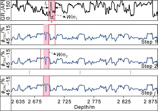
Fig. 5. Similar feature matching process between target well log (ϕCNL) and reference well log (GR1). |
Table 2. Average matching coefficients and standard deviations in the test set that capture similar feature sequences between well logs |
| Well number | GR1-GR2 | SP-GR1 | Δt-GR1 | ϕCNL-GR1 | ρ-GR1 | RLLD-GR1 | RLLS-GR1 | |||||||
|---|---|---|---|---|---|---|---|---|---|---|---|---|---|---|
| R | σ | R | σ | R | σ | R | σ | R | σ | R | σ | R | σ | |
| L1-9 | 0.89 | 0.20 | 0.38 | 0.42 | 0.68 | 0.27 | 0.46 | 0.34 | ||||||
| S2-16 | 0.86 | 0.24 | 0.31 | 0.46 | 0.65 | 0.31 | 0.40 | 0.39 | 0.49 | 0.26 | 0.48 | 0.27 | ||
| L1-10 | 0.91 | 0.21 | 0.79 | 0.32 | 0.36 | 0.40 | 0.73 | 0.25 | 0.49 | 0..35 | 0.50 | 0.26 | 0.50 | 0.25 |
| L1-11 | 0.87 | 0.23 | 0.33 | 0.44 | 0.67 | 0.28 | 0.43 | 0.36 | 0.53 | 0.22 | 0.52 | 0.24 | ||
3.3. Prediction results of depth matching of multi-well logs based on DDQN
A one-dimensional CNN sliding window convolves the feature sequences on well logs and inputs them into the MARL model for learning. After multiple rounds of training, the trained model is used to predict depth matching on a new test set. Fig. 6a shows the training performance of the agent in the environment, where the training error rapidly decreases in the initial stage and gradually diminishes and stabilizes in later stages. This indicates that the model has quickly learnt to utilize the optimization strategy for depth matching through feedback signals in the initial stage, and it’s finely tuned in the subsequent stages. The decreasing value and amplitude of the loss function learned by the agent in the environment suggest improved learning effectiveness. Fig. 6b displays the reward function obtained during the training process on the training set, reflecting the optimization effect of the depth matching task. The reward function starts at a lower value, gradually increases over time steps, and eventually stabilizes around 0.834, indicating that the correlation between the predicted depth of the well log and the real depth is gradually enhanced in the process of training the model, and the learning effect is better. Fig. 7 illustrates the depth matching prediction result for Well L1-11 in S Oilfield. Comparing the depth differences between the original and matched well logs, the DDQN algorithm successfully captured the most similar feature sequences on the target well logs (GR2, ϕCNL, ρ, etc.) and the reference well log (GR1). The corrected target well logs are well aligned with the reference well log, especially in the significant feature sequences (Fig. 7 ). The red boxes at the same depth positions on the well logs in Fig. 7 illustrate the significant effect of depth matching before and after using the DDQN algorithm, indicating that the well logs have been improved after DDQN depth matching.
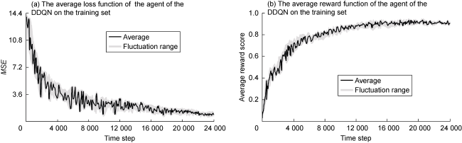
Fig. 6. Average loss function and average reward function of the agent on training set based on the DDQN. |
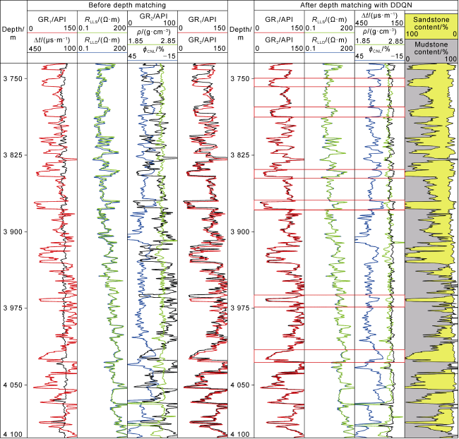
Fig. 7. Depth matching results of multiple well logs using DDQN in Well L1-11. |
3.4. Comparative analysis of predicted results from different methods
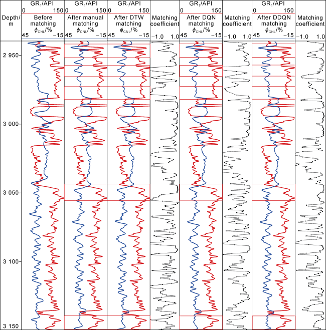
Taking another well, L1-10, as a case, we compared the depth matching prediction results of DTW, DQN, and DDQN methods, and the manual matching results through CIFLog software. The prediction results before and after depth matching between GR2 and GR1 are depicted in Fig. 8 , while the depth matching results between ϕCNL and GR1 are shown in Fig. 9. As can be seen from Figs. 8 and 9 , the DDQN captured significant similar feature sequences (in the red boxes) on the target well logs (GR2, ϕCNL) and the reference well log (GR1). Moreover, the overall predicted matching effect by DDQN is better than manual matching, DTW and DQN, and reducing the manual intervention. The depth matching effect of GR in Fig. 8 is better than that of ϕCNL in Fig. 9 , maybe due to GR and ϕCNL measuring different physical properties of the formation. GR measures the content of natural radioactive elements, whereas ϕCNL measures the hydrogen content in formation. These two types of properties have discrepancy in physical signals. All GR logs record the same parameter of natural radioactivity, making similar physical signals easier to be captured. Fortunately, the DDQN algorithm can capture most similar feature sequences, so its matching accuracy is high (Fig. 9 ). DTW performs well on simple feature sequences, but struggles with complex sequences, especially those with strong nonlinear features (at depth around 3 055 m and 3 140 m in Fig. 8 ). Although DQN performs better than DTW on the sequences with significant changes in the nonlinear feature, the former is still affected by overestimation of the Q-value, resulting in slight discrepancies between the target and the reference well logs (at depth near 3 055 m in Fig. 8 and 2 965 m in Fig. 9 ). All the prediction models used in this study were run on a computer with a 4.90 GHz Intel i7-12700 CPU and an NVIDIA GeForce 3 080 graphics card. As shown in Table 3 , DDQN spent longer time than DQN, which is 23.26 min and 16.53 min, respectively. Table 3 also summarizes the evaluation results of similar features captured by different methods based on dual sliding window after depth matching on the test set. The statistical prediction results in Table 3 indicate that all the methods generally achieved good depth matching effects, but R, MAE, and R2 of the DDQN method are superior to those of DQN and DTW. The prediction effect of DQN on the test set still lags behind DDQN, with minor discrepancies between the target well log and the reference well log near complex feature segments in Figs. 8 and 9 , suggesting that DDQN performs better than DQN in matching effects and error reduction.
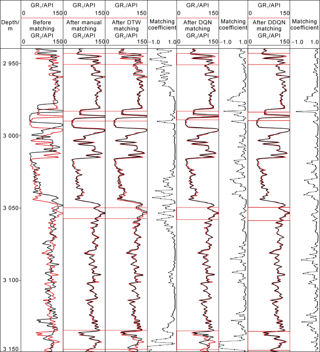
Fig. 8. Depth matching results of GR2 and GR1 using different methods in Well L1-10. |
Table 3. Evaluation results of different depth matching methods |
| Method | R | MAE | R2 | MSE | Reward | Time/min |
|---|---|---|---|---|---|---|
| DTW | 0.801 | 0.635 9 | 0.783 | 0.462 7 | ||
| DQN | 0.836 | 0.509 2 | 0.807 | 0.291 4 | 0.715 | 16.53 |
| DDQN | 0.884 | 0.393 4 | 0.816 | 0.176 2 | 0.793 | 23.26 |
Fig. 9. Depth matching results of ϕCNL and GR1 using different methods in Well L1-10. |
4. Conclusions
This paper proposes a MARL method for automatic depth matching of well logs, which was applied in S Oilfield. The methodology proceeds as follows: First, a variable one-dimensional CNN dual sliding window is used to extract feature sequence signals from the well log from top to bottom to capture the feature sequences on the target well log similar to those on the reference well log based on the principle of spatial similarity. Second, the DDQN algorithm, based on the Q-value function, is employed to address depth correction. The agent observes the matching state of similar features within the dual sliding window in the environment and uses an ε-greedy strategy to select the action corresponding to the maximum Q-value function, either translating or scaling the feature sequences to achieve desired matching effects. The DDQN algorithm incorporates the advantages of the DQN algorithm by introducing a dual-network structure for automatic depth matching tasks, where actions are selected through the evaluation network, and their Q-values are calculated through the target network, preventing overestimation of Q-values. Furthermore, a high-dimensional action space (by translating or scaling) and the Akima interpolation function are introduced to accomplish depth matching of multiple well logs. It can realize complex depth alignment, adjustment of depth deviation, and reduce the difficulty in selecting the initial state, and consequently enhancing the prediction accuracy of the algorithm.
Application of DTW, DQN and DDQN in a well in S Oilfield found that DTW can measure the time series similarity between two well logs and performs well in depth matching between two well logs, but is incapable of processing multiple well logs simultaneously. DTW is suitable for depth matching between GR curves with similar time series because it lacks a capability to learn or adapt to new conditions, and “lags” when encountering complex feature sequence segments on other target well logs. DQN and DDQN can keep learning with the interaction between the agent and the environment, and they have strong capabilities to learn and adapt to new matching tasks. DQN and DDQN learn the feature sequences of the reference well log with no need of extensive data labeling, and can handle depth matching tasks for multiple wells and multi-well logs simultaneously. However, DQN overestimates the action value function (Q) when matching complex feature sequences on well logs, which may lead to instability in the learning process and slight discrepancies in prediction results. The DDQN algorithm that employs a dual-network evaluation mechanism makes some improvements on DQN. It can provide better matching results although it consumes a slightly longer time.
5 Nomenclature
a, a°—the action taken by the agent at present time step and next time step;
argmax—argmax function;
—the action taken by the ith agent at time step t, i=1, 2, …, N;
—the ordinate of point , , k=1, 2, …, N;
—the action space taken by the multi-agent system at time t;
—coefficient in the Akima interpolation function;
—element in the ith row and jth column of matrix ;
—cost matrix in DTW algorithm;
, —the second and third derivatives of the Akima interpolation function at point xk in the kth segment of the curve;
—the Euclidean distance between points xi and yj in a matrix, ;
—expectation operator;
GR—natural gamma ray, API;
Loss—Loss function;
lt—length of sequence feature segment within the sliding window at time t, m;
min—the minimum cumulative Euclidean distance function in DTW;
—the optimum action selected by the agent under state s°;
—the slope calculated from the endpoints of the kth segment of the curve within the sliding window;
MAE—mean absolute error;
, —number of sampling points within the sliding window, , ;
, —upper and lower boundaries of the sliding window;
N—total number of agents;
—set of mapping strategies from the environmental state to the action taken by the multi-agent system at time t;
—Q-value function;
R—matching coefficient;
R2—coefficient of determination;
—reward space obtained by the multi-agent system at time t;
—reward obtained by the ith agent at time step t;
RLLD—deep lateral resistivity, Ω·m;
RLLS—shallow lateral resistivity, Ω·m;
s, s°—matching states of well log at the current and next time steps;
softmax—probability distribution function of machine learing classification;
—matching state of the well log observed by the ith agent at time step t;
SP—spontaneous potential, mV;
—set of state space of the well log observed by the multi-agent system at time t;
t—time step;
—mean depth of sampling points on the target well log,;
—mean depth of sampling points on the reference well logm;
Win1, Win2—dual sliding windows;
xi—depth of the ith sampling point on the reference well log, m;
xj—The depth of the jth sampling point on the target well log, m;
X={x1, x2 ,…, xn}, Y={y1, y2,…, yn}—set of sampling points on the two well logs;
—true depth of the ith sampling point on the reference well log, m;
—predicted depth of the ith sampling point in the similar feature sequence on the target well log, m;
α, β—weight of the reward function of depth matching, α=1.1, β=2.3;
—mapping strategy of the Nth agent from state st,i to action at,i at time t;
γ—discount factor;
θ—weight of the current evaluation network;
θ°—weight of the evaluation network after state update;
—weight of the target network after state update;
ϕCNL—compensated neutron porosity, %;
ϕpredict—predicted depth values of the target well log during depth matching by the agent, m;
ϕtrue—actual depth values of the reference well log, m;
ρ—density, g/cm3;
—learning rate;
Δ—sampling interval, Δ=0.125 m;
Δt—acoustic time difference, μs/m;
—gradient of the Q-value function with respect to parameter θ;
—weight of Akima interpolation function;
, —coordinates of the endpoints of the kth segment of the well log when using Akima interpolation;
(x, S(x))—coordinates of an interpolation point on the kth segment within the sliding window.