

Introduction
Shale reservoirs have extremely low permeability and require hydraulic fracturing stimulation to realize commercial exploitation. Hydraulic fracturing stimulation is a process not only creating fractures, but also inducing the redistribution of reservoir fluid, resulting in local high pressure and affecting post-fracturing production of shale gas wells [1]. Currently, the most common integrated simulation of fracturing and production first obtains parameters such as fracture geometry and conductivity through hydraulic fracturing simulation, and then imports these fracture parameters into a production simulator to simulate post-fracturing production. Xu et al. [2] set all grids boundaries as cohesive elements to consider the offset of hydraulic fractures during fracture network simulation. They incorporated the fracture geometry pa-rameters derived from fracturing simulation into an embedded discrete fracture model (EDFM) which accounts for matrix nonlinear flow, etc., to predict the post-fracturing production of tight oil. Sherratt et al. [3] used the finite element method to obtain fracture geometry, and then directly modified the matrix model via equivalent permeability to complete numerical simulation of post- fracturing production. Xia et al. [4] employed a multiple continuous/discrete fracture model to simulate the post- fracturing production of shale gas reservoirs. Zhao et al. [5] used an EDFM to simulate the post-fracturing production of marine-to-terrestrial transitional shale gas reservoirs. Due to the difference in data structure among simulators, the fracture data obtained from fracturing simulation need to be processed before they are applied to reservoir production models, which significantly limits their application. In order to further strengthen the coupling between fracturing and production, Weng et al. [6] developed a Kinetix fracturing-production integrated numerical simulation platform based on the Petrel system to solve the problem arising from cross-environment and cross-system conversion between fracturing and production models. This method has been widely applied in shale oil and gas fields [7]. Cao et al. [8] utilized a discrete fracture network (DFN) to depict the fracture geometry calculated using the displacement discontinuity method (DDM), and preliminarily achieved the integration of fracturing and production simulation by combining DDM with discrete fractures. However, this process is only one-way simulation and can not realize the coupled simulation of fracture propagation and reservoir fluid flow. Chang et al. [9] also combined DDM (to simulate fracture propagation) with EDFM (to simulate production) and used the ZFRAC software to internally transfer fracturing results to production process. The FrSmart software developed by PetroChina Research Institute of Exploration and Development also implements integrated fracturing and production simulation through inter-module data transfer [10]. Implementing simulation from fracturing to production in the same system can effectively reduce numerical calculation errors caused by model conversion. However, the methods above do not consider the changes in matrix pore pressure and two- phase flow in reservoirs caused by hydraulic fracturing.
The influence of pore pressure on fracture propagation is manifested in two aspects. Firstly, due to poroelastic effect, the increase in pore pressure around fractures changes the stress state, affecting fracture deformation and propagation. Secondly, the increase in pore pressure affects the rate of fluid loss inside fractures, thereby impacting the propagation process. Some researchers simulated the fluid-solid coupling between matrix and fracture in the process of fracture propagation within a single-fluid system through different methods. Due to the large computational demand of such models, they have not yet been applied to practical field operation. Wang et al. [11] considered the similarity of model structures between extended finite element method (XFEM) and EDFM, and combined them to achieve flow-solid coupled simulation between matrix and fracture in the process of single-phase fluid and single-fracture propagation when the effect of pore pressure variation on fracture propagation was considered. Based on the finite-discrete element method (FDEM), Yan et al. [12] considered the change of reservoir pore pressure in the process of single fracture propagation. In addition, some researchers used continuous mechanics methods considering rock damage [13], discontinuous discrete models [14], lattice methods based on discrete elements [15-16], and DDM-EDFM coupling methods [17] to simulate the change in matrix pore pressure during fracturing process. These works primarily focused on analyzing the changes in pore pressure during fracturing, but less considered post-fracturing production.
The fluid used for fracturing shale gas reservoirs is mainly slickwater, while original pore fluid is mainly methane. Gas-liquid two-phase flow is common during hydraulic fracturing. In the presence of multiphase fluids, the difference in compressibility between different phases always influences fracture propagation. Park et al. [18] found that fluid compressibility is inversely proportional to hydraulic fracture length. When matrix has lower water saturation, the overall compressibility of reservoir fluid is higher, resulting in slower fracture propagation. Since there may be a certain distance between the front of fracturing fluid and fracture tip, a pseudo vacuum area may appear at fracture tip. Yoon et al. [19] used a fully coupled multiphase flow and fracture propagation method to analyze the size of the vacuum area and dry area at fracture tip. They believed that rock compressibility, permeability, and fracture compressibility are key factors controlling the dryness of the tip area, and high matrix permeability may result in a slower increase in water saturation and fracture length at the injection point. Based on a phase field approach, Lee et al. [20] also developed a numerical simulation method coupled with matrix and two-phase flow, and carried out simulation analysis of the process of fracturing fluid flowback. Zheng et al. [21] realized the simulation of thermal-fluid-solid coupled fracture propagation considering multiphase flow based on the finite element method. The model assumes that fractures extend along multiple parallel planes in a fixed direction. For the problem of non-planar fracture propagation when multiphase flow is considered, Ren et al. [22] coupled XFEM with EDFM to simulate the bending and propagation process of multiple fractures under stress interference, which emphasized the impact of poroelastic effect on oil production after fracturing operation. Due to the difficulty in constructing a crossing fracture enhancement function with XFEM, it is challenging to apply it to shale gas reservoirs with natural fractures. Existing fracturing models considering gas-water two-phase flow still mainly focus on small-scale mechanism models, but less on field-scale fracture network simulation. The aforementioned studies focused on fracturing process, but less considered simulation on the integrated fracturing-production process.
In this paper, we use the unified pipe-network method (UPM) constructed by Ren et al. [23-24] to characterize the gas-water two-phase flow in fractures and matrix, use the DDM to calculate the deformation and propagation direction of fractures, and construct an integrated fracturing-production numerical model by sequential iteration considering gas-water two-phase flow. This model considers the influence of natural fractures and matrix properties on fracturing process, and directly uses the distribution of formation pressure and water saturation after fracturing operation for subsequent well soaking and production simulation, achieving continuous simulation of the entire development cycle from fracturing to production.
1. Integrated numerical model for fracturing and production
1.1. Model establishment
In our model, we assume the fracturing fluid injected into formation is clear water (namely, no filter cake induced), which can be approximately deemed equivalent to low-viscosity slickwater. If field fracturing operation employs high-viscosity fluid like guar gum, it is necessary to differentiate among formation water, fracturing fluid and natural gas, and construct a new flow model. Shale matrix is extremely tight with poor pore connectivity, and the poroelastic effect is weak. The stress induced by the change of pore pressure around fractures is smaller than the stress induced by the fractures themselves, so the poroelastic effect is neglectable. Moreover, it is assumed that the pressure inside a horizontal wellbore is uniform, and surface production is calculated from subsurface gas and water production using a volume factor, without considering the impact of tubing flow inside the wellbore.
The discrete fracture model facilitates multiphase flow simulation in fractures and matrix by reducing fractures to one-dimensional line elements. Similarly, the hydraulic fracturing model based on DDM also represents fractures as one-dimensional line elements. Thus, it is feasible to couple these two methods. The UPM model developed by Ren et al. [23-24] based on the concept of discrete fractures and reduces the flow in both matrix and fractures to one-dimensional pipe model, thus significantly enhancing computational efficiency. The flow between pipelines is characterized by the nodes at both ends of the pipeline, and the activation of the nodes is used to characterize the propagation of fractures, which has a good adaptability to dynamic fracture propagation. Therefore, this paper constructs an integrated fracturing-production numerical model by coupling the UPM model with the DDM model.
In the integrated fracturing-production numerical simulation process constructed in this paper (Fig. 1 ), first, the UPM model is used to calculate the fluid pressure and saturation within fractures and matrix after injecting fracturing fluid at the current time step, then the DDM model calculates the displacement discontinuity of the fracture elements based on the fracture pressure provided by the UPM model. Based on the displacement discontinuity of the fracture elements, fracture propagation is assessed, and fracture permeability is updated. If the fracture tip does not meet the quasi-static extension criteria, the time step is dynamically adjusted, and the computation is restarted. The two-phase flow and fracture aperture calculations are coupled using a sequential iterative approach. The core of this model is the dynamic updating of fracture aperture and permeability in the UPM model. The UPM model transfers the internal fracture pressure to the DDM model, and the DDM model transfers the fracture aperture back to the UPM model. In the fracture propagation process, initially, all grid cells are assumed to be potential fractures, with the same permeability as the matrix and in an inactivated state. When the fracture extension criterion determines that a cell is activated, it is considered a fracture cell, and the DDM model is used to update the permeability between fracture nodes. The model in this paper is implemented through custom programming in MATLAB, currently running on a standalone version without external dependencies.
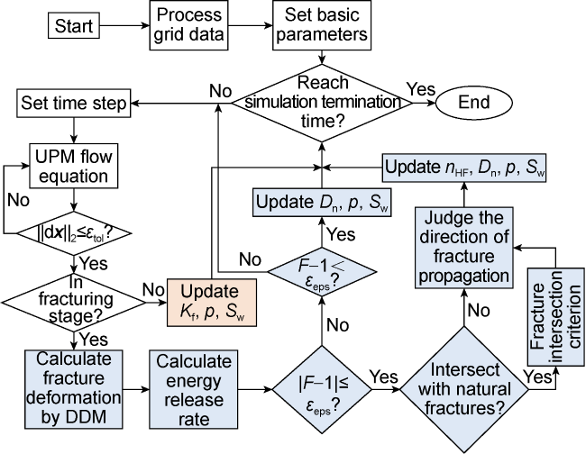
Fig. 1. Integrated fracturing-production numerical simulation process. |
1.1.1. Gas-water two-phase flow characterization
The UPM model characterizes the flow process by superimposing the flow potentials in matrix and fractures at the same location, with no need to construct a channeling term to represent the flow between the two systems.
The two-phase flow equations for matrix system are as follows:
The two-phase flow equations for fracture system are as follows:
For any given matrix triangular element in the UPM model using unstructured grids (Fig. 2a ), when the control volume discretization is applied, the control volume at each node is the volume enclosed by the circumcenter of the triangle and the node (Fig. 2b and Eq. (3)).
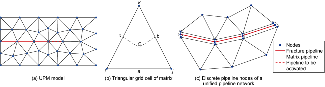
Fig. 2. Schematic diagram of UPM model. |
To allow hydraulic fractures to extend along any grid boundary, it is assumed that each control node has three flow channels (Fig. 2c ), of which two are matrix channels and one is a fracture channel. The seepage flow of the three channels is superimposed to represent the cumulative seepage flow at the current control node. Through this method, it is not necessary to dynamically adjust the number of flow channels in subsequent simulations, which keeps the equation structure unchanged and thus improves model computational efficiency. For units that have not been fractured, the fracture channel has no permeability. For units that have been opened, the permeability of the fracture channel is calculated based on the aperture of the fracture channel obtained using the DDM, that is:
The flow in the matrix system is solved using the finite element method, and the permeability between nodes in Fig. 2b can be represented as:
In addition, considering the difference between the matrix system and the fracture system, the conversion of water saturation between the two systems is achieved by using the same capillary pressure at the interface between the fracture and matrix, which can be expressed as follows [25]:
By combining the above equations and using Newton iteration for fully implicit solution, the pressure and saturation of the reservoir at any point at any injection time during fracturing can be calculated.
1.1.2. Fracture deformation characterization
This paper uses a two-dimensional DDM model to calculate the deformation and propagation of fractures under fluid pressure inside the fracture and external stress. The model has been introduced and validated in details in previous work [26], so it is only explained in brief. In the two-dimensional DDM model, the fracture element is one-dimensional line segment, and each element has two unknown variables to be solved: normal displacement discontinuity and tangential displacement discontinuity. The discontinuous displacement of each element is calculated based on the stress balance relationship of each element, that is, the internal force of the fracture element is equal to the external load (the sum of induced stress and far-field stress of other elements)
In Eq. (7), σn,α and τs,α respectively represent the normal stress and the shear stress on fracture element α. For a hydraulic fracture, σn,α is equal to the fluid pressure inside the fracture (the average pressure of the two phases in the fracture pipeline calculated based on the UPM model), τs,α is zero. σn0,α and τs0,α represent the far-field normal and shear stresses on fracture element α, respectively. Ass,αβ, Asn,αβ, Ans,αβ, and Ann,αβ are the stress influence coefficients of fracture element β on element α. Gαβ is the three-dimensional fracture height correction factor for the induced stress of fracture element β on element α, and the specific expression and algorithm can be found in Reference [26]. Ds,β and Dn,β are the shear and normal displacement discontinuities of fracture element β, which are unknown in Eq. (7). Dn,β is fracture aperture, which can be transmitted to the fracture aperture w in Eq. (4) to achieve coupling between fracture deformation and flow inside fractures.
By solving Eq. (7), the displacement discontinuity of a fracture element under fracture pressure at the current time step can be obtained, and then the change in fracture aperture can be calculated.
1.1.3. Fracture propagation characterization
The stress intensity factor at fracture tip can be expressed as:
where .
When the energy release rate at fracture tip reaches the critical rate (G=GIC), fracture extends and the front-end fracture pipeline unit is activated. The direction of fracture propagation is the direction with the highest energy release rate, and the equation for calculating energy release rates in different directions is:
where
$\begin{array}{l} K_{\mathrm{I}}^{*}(\theta)=\frac{4}{3+\cos ^{2} \theta}\left(\frac{\pi-\theta}{\pi+\theta}\right)^{\frac{\theta}{2 \pi}}\left(K_{\mathrm{I}} \cos \theta-\frac{3}{2} K_{\mathrm{II}} \sin \theta\right) \\ K_{\mathrm{II}}^{*}(\theta)=\frac{4}{3+\cos ^{2} \theta}\left(\frac{\pi-\theta}{\pi+\theta}\right)^{\frac{\theta}{2 \pi}}\left(K_{\mathrm{II}} \cos \theta+\frac{1}{2} K_{\mathrm{I}} \sin \theta\right) \end{array}$
The simulation method of hydraulic fracture propagation in UPM model (Fig. 3 ) assumes that fractures extend along grid boundaries, and when the fracture tip encounters the discrete grid element ahead, the fracture will form multiple angles with different boundaries (θ1, θ2, θ3, θ4 in Fig. 3a ). Each boundary is a potential direction for fracture propagation. Firstly, the energy release rate of the hydraulic fracture propagation at each angle is calculated, and the matrix unit that reaches the critical energy release rate and of the maximum value is the next fracture propagation target. Based on the above criterion, fracture deflection can be realized. The fracture paths corresponding to different gridding methods are shown in Fig. 3b-3d . It can be seen that under the premise of high-quality gridding, the fracture propagation path is relatively stable.
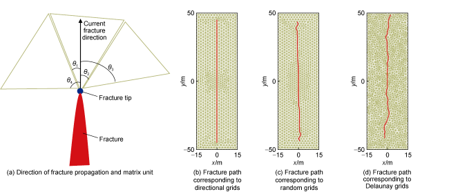
Fig. 3. Schematic diagram of the fracture propagation simulation in UPM model. |
This study assumes that fracture propagation satisfies quasi-static conditions and dynamically adjusts the time step during simulation to achieve a quasi-static propagation process. An initial time step (5 s in this paper) is used to simulate the injection of fracturing fluid, obtaining the distribution of pressure and aperture within the fracture. When the fracture tip meets the propagation criterion (G=GIC) under this time step, the fracture advances by one unit; if G>GIC, the time step is shortened and the simulation is redone; if G<GIC, the process proceeds to the next time step, continuing the injection of fracturing fluid until the fracture propagates.
In this paper, natural fractures are considered as weak planes, with a lower critical energy release rate along the direction of the natural fractures. Whether hydraulic fractures cross natural fractures depends on the ratio of the energy release rate to the critical energy release rate along a channel element [27].
1.1.4. Calculation of fracture permeability during well soaking and production
Assuming that proppants are uniformly placed inside fractures when they stop propagating. The initial aperture of a fracture is the aperture when the fracture stops propagating. The fracture is considered to be closed during well soaking and production, and the permeability change after fracture closure is related to the initial fracture aperture and effective stress. The permeability at different fracture apertures can be obtained based on the results of fracture stress sensitivity experiments. Further, according to the experimental results of fracture permeability under different effective stresses, the relationship between the fracture permeability and effective stress under different initial fracture apertures can be obtained.
Taking the Silurian Longmaxi shale in the Sichuan Basin as an example, the permeability of cores with sand-filled fractures of different apertures under different confining pressures was determined through the stress sensitivity experiment on propped fracture conductivity. Test groups were selected with effective stresses (the difference between the normal stress on the fracture and the fluid pressure inside the fracture) of 10, 20, 30, 40, 50 and 60 MPa, and a graph showing the relationship between fracture aperture and permeability was plotted (Fig. 4a ).

Fig. 4. Relationship of permeability with fracture aperture (a) and empirical coefficients at different stresses (b). |
According to Fig. 4a , under different effective stresses, the permeability of sand-filled fractures and the fracture aperture exhibit a clear logarithmic relationship, which can be expressed as follows:
The relationship between effective stress and coefficients A and B in Eq. (11) can be obtained through further fitting (Fig. 4b ). Consequently, an empirical relationship between propped fracture permeability, fracture aperture, and effective stress can be derived as follows:
The error between Eq. (12) and actual result is controlled within ±5%, which proves the rationality of the empirical relationship equation fitted in our paper.
The formation pore pressure, water saturation, and fracture aperture after fractures stop expanding are adopted as the initial state of production simulation, thus realizing the close integration of fracturing and production processes. In addition, the fracture parameters, reservoir pressure field, and fluid field obtained under the premise of gas-water two-phase flow under the coupling of matrix and fractures in the fracturing process can be accurately applied in the numerical simulation of oil and gas reservoirs.
1.2. Model validation
Simulation results of oil-water two-phase flow established by Monteagudo et al. [25] based on a discrete fracture model are used to validate the multiphase flow characterization method of the model in this paper. The parameter settings are consistent with those in Reference [25]. The density of the oil phase is 600 kg/m3, and the viscosity is 0.45 mPa·s. The density of the water phase is 1 000 kg/m3 and the viscosity is 0.80 mPa·s. The model size is 1 m×1 m, the matrix porosity is 20%, and the permeability is 1×10⁻³ μm2. The fracture aperture is 0.1 mm, the porosity is 100%, and the permeability is 8.26×10⁻¹⁰ m2. One water injection well is in the lower left corner of the model, and one production well is in the upper right corner. Assuming that both oil and water are incompressible fluids, the flow rate in both the production well and the injection well is 2.32×10⁻⁸ m3/s, namely 0.01 PV/d (PV means pore volume). As can be seen from Fig. 5 , the water saturation distribution calculated by this paper's method is more consistent with the simulation result in Reference [25], which verifies the accuracy of this paper's model in the characterization of multiphase flow.
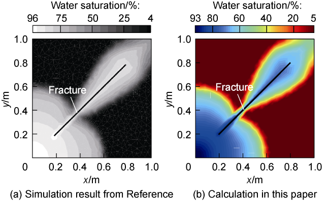
Fig. 5. Simulation of water saturation distribution from Reference [25] and calculation in this paper. |
The single-fracture propagation model based on the DDM has been validated in our previous work [26]. Here, the simulation result of fracture propagation based on multiphase flow is verified. Assuming that the relative permeability curves of matrix and fractures are both "X" type, the main model parameters are shown in Table 1. A numerical model with a calculation range of 90 m×20 m is constructed for hydraulic fracturing numerical simulation, and the initial fracture length is 10 m (Fig. 6a ).
Table 1. Parameter settings for model validation |
| Parameter | Value | Parameter | Value |
|---|---|---|---|
| Matrix porosity | 10% | Elastic modulus | 40 GPa |
| Matrix permeability | 0.000 1× 10⁻³ μm2 | Poisson's ratio | 0.25 |
| Initial formation pressure | 25 MPa | Reservoir thickness | 20 m |
| Irreducible water saturation | 20% | Viscosity of fracturing fluid | 5 mPa·s |
| Maximum horizontal principal stress | 35 MPa | Injection rate | 0.02 m3/s |
| Minimum horizontal principal stress | 30 MPa | Fracture toughness | 1.5 MPa·m1/2 |
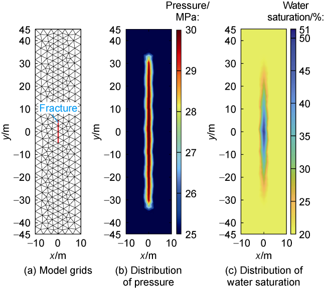
Fig. 6. Model grids and distribution of pressure and water saturation at the end of simulation. |
According to the dimensionless parameter , the fracture propagation in the case is controlled by viscosity, and the analytical solutions to the half-fracture length and the pressure at the injection point are [28]:
As can be seen from Fig. 7 , the numerical simulation results of hydraulic fracture propagation coupled with multiphase flow in this paper are closer to the analytical solutions. Since the matrix permeability is small in this case, the actual fracture propagation results are more consistent with the analytical solutions. Since the simulation of fracture propagation is in the form of unit activation, the growth of fracture length is in the form of steps. Using the model in this paper, matrix pressure and water saturation distribution can be obtained simultaneously during fracture propagation (Fig. 6b , 6c ). In this example, only the matrix grid cells adjacent to fractures show significant changes in pressure and water saturation.
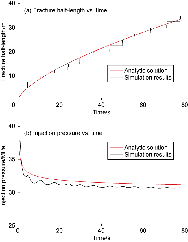
Fig. 7. Simulated results of fracture half-length and injection pressure compared with analytical solutions. |
2. Numerical simulation of fracturing-production integration
2.1. Model settings
Based on the above integrated numerical model, integrated fracturing-production simulation analysis considering gas-liquid two-phase flow is carried out. The model parameters are shown in Table 2. The model size is 50 m×150 m. The relative permeability curves of matrix and fracture are shown in Fig. 8a . It is assumed that the fracture and the matrix have the same capillary pressure (namely, the coefficient of the fitting formula for capillary pressure is 0.3), and the irreducible water saturation in the matrix is 30%. The initial grid of the model and the distribution of fractures are shown in Fig. 8b .
Table 2. Parameter settings for integrated fracturing-production simulation model |
| Parameter | Value | Parameter | Value |
|---|---|---|---|
| Matrix porosity | 10% | Elastic modulus | 40 GPa |
| Matrix permeability | 0.000 5× 10⁻³ μm2 | Poisson's ratio | 0.2 |
| Initial formation pressure | 45 MPa | Porosity of fractures | 50% |
| Initial water saturation in matrix | 40% | Wellbore radius | 0.1 m |
| Initial water saturation in fracture | 10% | Injection rate | 5 m3/min |
| Maximum horizontal principal stress | 32 MPa | Natural fracture aperture | 0.1 mm |
| Minimum horizontal principal stress | 30 MPa | Reservoir thickness | 20 m |
| Type I fracture toughness of matrix | 5 MPa·m1/2 | Viscosity of fracturing fluid | 0.3 mPa·s |
| Type I fracture toughness of natural fracture | 3 MPa·m1/2 | Fracturing duration | 1.5 min |
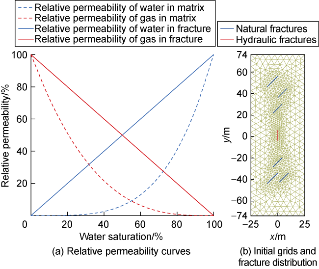
Fig. 8. Relative permeability curves, initial grids, and fracture distribution. |
2.2. Fracturing simulation
2.2.1. Simulation of fracture propagation process
The effect of formation water saturation on fracture propagation isn’t considered in the fracturing model under conventional single-phase flow assumption. In this paper, the initial water saturation in matrix is set to 30%, 40% (base case) and 50% to carry out hydraulic fracturing simulation and analyze its influence on fracture propagation. As shown in Fig. 9 , with the increase of initial water saturation, the compression coefficient of the fluid in reservoir decreases, and pressure can transfer from the injection point to the fracture tip more quickly as fracturing fluid is injected, which results in rapid fracture growth. In addition, the higher the initial water saturation, the lower the matrix capillary pressure during fluid injection, and the more difficult it is for fracturing fluid to intrude into the matrix. At this time, the injected fluid tends to flow along the fracture, which also contributes to the rapid growth of the fracture. As can be seen from Fig. 10 , fracturing fluid is concentrated in the vicinity of the hydraulic fracture with limited total amount invaded. The higher the initial water saturation in the matrix, the smaller the increase of water saturation near the fracture is, which is consistent with the analyzed results in Fig. 9 .
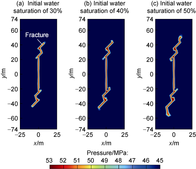
Fig. 9. Post-fracturing pressure distribution at different initial water saturations of matrix. |
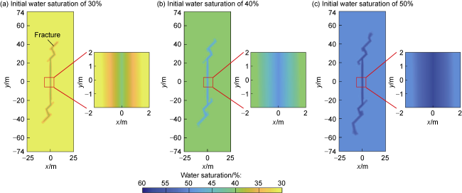
Fig. 10. Post-fracturing water saturation distribution at different initial water saturations of matrix. |
2.2.2. Simulation of pump-stopping stage
Due to the extremely low permeability of shale matrix and the slow leak-off of fracturing fluid, the fracture can keep propagating after stopping the pump. As can be seen from Fig. 11 , after the end of fracturing, there is still a pressure gradient from the injection point to the fracture tip, which makes fracturing fluid continue moving to the fracture tip, and in turn, fracture propagation continues, and the pressure gradient decreases until the propagation stops. In this example, the fracture can keep growing 5-15 m after stopping the pump.
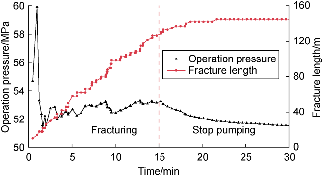
Fig. 11. Changes in bottomhole pressure and fracture length before and after pump-stopping. |
2.3. Simulation of production processes
It is assumed that the well is shut in for 30 d after fracturing, and then the well is opened for production for 15 years at fixed bottomhole pressure of 15 MPa. Fig. 12a shows the pressure changes at the injection point located at the center of the model during fracturing, soaking and production, and Fig. 12b shows the corresponding distribution of model pressure and water saturation. The pressure and water saturation changes at different stages can be accurately characterized in the same system, which realizes the integrated simulation of fracturing-soaking-production considering two-phase flow.
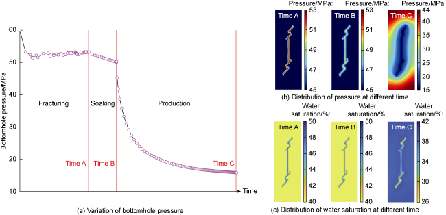
Fig. 12. Variation of bottomhole pressure at different stages and distribution of pressure and water saturation at different time. |
The difference in gas and water production performances obtained from different simulation methods were compared, including the simulation simultaneously considering the effect of fracturing process on matrix pore pressure and water saturation (integrated coupling), the simulation considering the effect of fracturing process on matrix pore pressure only (coupling pressure), and traditional production simulation only considering fracture parameters (no coupling) (Fig. 13 ). For traditional production simulation, the reservoir pressure and saturation fields are under original formation conditions, and the fractured wells have lower initial water production and lower ultimate cumulative gas production. For the method only coupling pressure, fracturing stimulation induces locally high pressure around the fracture, resulting in higher initial gas production, and the initial water production is also higher than that of the uncoupled method. For the integrated coupling method, fracturing stimulation induces locally high pressure around the fracture and also creates high water saturation near the fracture, and a large amount of fracturing fluid is retained at the bottom of the well. Therefore, the initial gas production effect is generally moderate, and rapid flowback of fracturing fluid brings higher initial water production, resulting in a significant increase in cumulative water production.
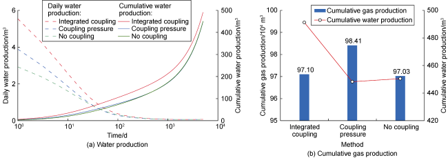
Fig. 13. Comparison of simulated water production and cumulative production using different methods. |
2.4. Field application
The model proposed in this paper was used for integrated fracturing-production simulation by taking a typical horizontal well H in Ning 201 well zone of the Changning shale gas area in the Sichuan Basin as a case. The target layer is the organic-rich shale in the Upper Ordovician Wufeng Formation and the lower member of the Lower Silurian Longmaxi Formation, Sichuan Basin. The shale interval is totally 30-50 m thick at 2 300 m to 3 200 m. The basic parameters of the reservoir are shown in Table 3.
Table 3. Basic parameters of the shale reservoir |
| Parameter | Value | Parameter | Value |
|---|---|---|---|
| Porosity | 6.8% | Elastic modulus | 40 GPa |
| Permeability | 0.000 102× 10−3 μm2 | Poisson's Ratio | 0.27 |
| Formation pressure | 55 MPa | Reservoir thickness | 30 m |
| Gas saturation | 68% | Rock density | 2.56 g/cm3 |
| Maximum horizontal principal stress | 73 MPa | Langmuir′s Volume | 3.48 m3 |
| Minimum horizontal principal stress | 63 MPa | Langmuir′s Pressure | 6.91 MPa |
The horizontal section of Well H is 1 500 m long, and fractured in 18 stages spaced by 80 m, and 3 clusters a stage. The operation pressure fluctuated in a small range after breakthrough, and then became stable overall, indicating a relatively uniform distribution of reservoir stress, and hydraulic fractures were not significantly affected by natural fractures during their propagation. From a computational standpoint, the impact of natural fractures on hydraulic fracture propagation in Well H was not considered.
Based on the model proposed in this paper, the average fracture length in Well H is about 220 m. In addition, the distribution of pressure and water saturation at different stages was calculated. From Fig. 14a and 14c, it can be seen that at the end of fracturing, the pressure near the fracture was higher than the matrix pressure. Meanwhile, the pressure at the injection position in horizontal well (i.e., the injection point) located in the middle of the fracture was higher, the pressure at the tip of the fracture was relatively low, and fracturing fluid was mainly distributed along the direction of the fracture. As can be seen from Fig. 14b and 14d, the pressure at the fracture location was lower at the end of production. Meanwhile, gas in the matrix flowed toward the fracture during steady production, and the matrix pressure around the fracture decreased. Water saturation around the fracture changed, but almost did not at other locations.
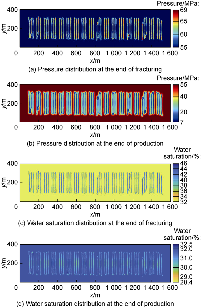
Fig. 14. Pressure and water saturation distribution in Well H at different stages. |
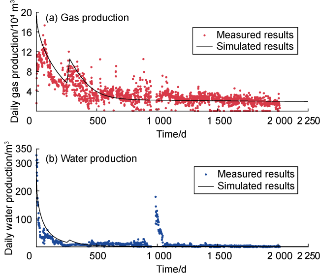
The model proposed in this paper was used to simulate the production performance of Well H (Fig. 15 ). The simulated result is almost consistent with the measured production data from the basic characteristics of the actual production data and the trend of the fitted curves.
Fig. 15. Fitting results of simulated and measured production performances of Well H. |
The error of cumulative gas production is 10.32%, and that of cumulative water production is 6.39%, which further verified the accuracy of our model. Based on the simulated production performance, the ultimate cumulative gas production is predicted to be 1.28×10⁸ m3 if the well continues to produce for 15 years with the current production regime.
3. Conclusions
The integrated fracturing-production numerical model considering gas-water two-phase flow proposed in this paper can provide the pore pressure and water saturation distribution of the formation after fracturing while predicting the fracture geometry. Therefore, the influence of matrix physical properties (e.g., water saturation) on fracturing process can be considered more rigorously. Compared with the conventional method, the model proposed in this paper can more accurately simulate the water and gas production by considering the effects of fracturing on matrix pressure and water saturation at the same time. Both the analysis of case studies and field application in a real horizontal well confirmed that the model is highly accurate
Due to the low permeability of shale matrix, fracturing fluid is mainly distributed along fractures, with a limited increase in matrix water saturation. After the end of fracturing operation, fractures can keep propagating a certain distance. Under the parameter conditions proposed in this paper, they can continue to extend for more than 10 m.
Nomenclature
A, B—empirical coefficients, m2;
Ass,αβ—the coefficient characterizing the shear stress induced by unit tangential displacement of fracture element β at the location of element α, dimensionless;
Asn,αβ—the coefficient characterizing the normal stress induced by unit tangential displacement of fracture element β at the location of element α, dimensionless;
Ans,αβ—the coefficient characterizing the shear stress induced by unit normal displacement of fracture element β at the location of element α, dimensionless;
Ann,αβ—the coefficient characterizing the normal stress induced by unit normal displacement of fracture element β at the location of element α, dimensionless;
Bf, Bm—capillary pressure fitting formula coefficients of fracture and matrix, dimensionless;
Bg, Bw—volume coefficients of gas phase and water phase, dimensionless;
—the two-norm of increment of an unknown at the current iterative step;
Dn—normal displacement discontinuity of a fracture element, m;
Ds—tangential displacement discontinuity of a fracture element, m;
Dα—tangential or normal displacement of fracture element α, m;
E—elastic modulus, Pa;
E°—plane-strain elastic modulus, Pa;
F—relative energy release rate, dimensionless;
G—energy release rate, N/m;
GIC—critical energy release rate, N/m;
Gαβ—three-dimensional fracture height correction factor under the induced stress from fracture element β to fracture element α;
h—fracture height, m;
K°—fracture toughness for asymptotic solution, Pa·m1/2;
Kf, Km—permeability of fracture and matrix, m2;
Kmp,ij—permeability between nodes i and j, m2;
Kmp,ik—permeability between nodes i and k, m2;
Kmp,jk—permeability between nodes j and k, m2;
Krfg, Krfw—relative permeability of gas phase and water phase in fractures, dimensionless;
Krmg, Krmw—relative permeability of gas phase and water phase in matrix, dimensionless;
Kα—stress intensity factor at the fracture tip of fracture element α, Pa·m1/2;
KI, KII—stress intensity factors at the tip of type I and type II fractures, Pa·m1/2;
l(t)—fracture half-length, m;
lij—distance between nodes i and j, m;
lik—distance between nodes i and k, m;
ljk—distance between nodes j and k, m;
lOa, lOb, lOc—distances between point O and points a, b, c, m;
Lf—half-length of a fracture element, m;
nHF—number of fracture elements;
p—fluid pressure, Pa;
p(0,t)—injection point pressure, Pa;
q—injection flow rate, m3/s;
qsg, qsw—gas and water source and sink terms, s−1;
Sw—water saturation, %;
Sfg, Sfw—gas saturation and water saturation in fractures, %;
Smg, Smw—gas saturation and water saturation in matrix, %;
t—time, s;
Vi, Vj, Vk—control volumes of nodes i, j, k, m3;
ViaOc—volume enclosed by the circumcenter O of triangular element and node i, m3;
VjaOb—volume enclosed by the circumcenter O of triangular element and node j, m3;
VkbOc—volume enclosed by the circumcenter O of triangular element and node k, m3;
w—fracture aperture, m;
α, β—serial number of fracture element;
εeps, εtol—tolerance factor;
θ—angle between potential and current propagation directions of a fracture, (°);
μ°—viscosity parameter for the derivation of asymptotic solution, Pa·s;
μg, μw—viscosity of gas phase and water phase, Pa·s;
σ—effective stress, Pa;
σn,α—normal stress on fracture element α, Pa;
σn0,α—far-field normal stress of fracture element α, Pa;
τs,α—shear stress on fracture element α, Pa;
τs0,α—far-field shear stress of fracture element α, Pa;
υ—Poisson's ratio, dimensionless;
Φfg, Φfw—potential energy of gas phase and water phase in fractures, Pa;
Φmg, Φmw—potential energy of gas phase and water phase in matrix, Pa;
ϕ—porosity, %;
ϕf, ϕm—porosity of fracture and matrix, %.