

Introduction
Spectral analysis in the time-frequency domain is an important technical means and tool for processing and analyzing non-stationary signals. It is frequently used in analyzing and processing seismic data [1]. By extending one-dimensional seismic data in the time domain into a two-dimensional time-frequency domain, it allows seismic data to be analyzed and processed in a higher dimensional space. This approach characterizes the information in the seismic data more effectively and thus helps in the exploration and development of oil and gas reservoirs.
Based on different mechanisms, conventional time-frequency analysis methods can be divided into linear and nonlinear time-frequency analysis methods. Typical candidates for linear time-frequency analysis methods are: Short-Time Fourier Transform (STFT) [2], Wavelet Transform (WT) [3], S Transform [4], W Transform [5], etc. Common nonlinear time-frequency analysis methods include the Wigner-Ville distribution (WVD) [6], the matching pursuit technique [7], and time-frequency analysis methods based on the reassignment of frequencies [8].
One of the most commonly used nonlinear time-frequency analysis methods for analyzing and processing seismic data is WVD [6]. The WVD can be expressed as the instantaneous cross-correlation between the complex signal and its conjugate signal and provides high resolution and energy concentration in the time-frequency spectrum. However, the cross-correlation between different signal components leads to significant crosstalk in the time-frequency spectrum. Various enhancement methods are aimed at suppressing this crosstalk. For example, the smoothed pseudo-WVD (SP-WVD) proposed by Choi and Williams [9] can effectively suppress crosstalk. The multi-channel WVD method with maximum entropy proposed by Wang et al. uses multiple WVD kernel functions to eliminate crosstalk between different components [10]. Rao et al. proposed to use the multi-channel maximum entropy WVD to estimate the dominant frequency of seismic data for identifying karst cavities in strata to improve the accuracy of seismic anomaly identification [11]. Alsalmi and Wang proposed the masked WVD method, in which a stable mask filter is constructed for post-processing the results of WVD time-frequency analysis [12]. These improved methods can all be regarded as filtering the time-frequency spectrum, which inevitably removes part of the valuable energy.
The problem of crosstalk in the WVD method can also be solved with the Matching Pursuit (MP) technique [13]. Wang introduced MP into seismic data processing and analysis and proposed the use of time-frequency spectrum when Morlet wavelets matching with seismic traces [7]. To improve the reliability of MP, Wang also proposed a multi-trace MP technique [14], which uses the average seismic trace between neighboring traces as a reference. This approach improves the lateral continuity of the time-frequency spectrum and suppresses random noises while increasing the convergence of MP. Zhao et al. proposed a structurally adaptive multi-trace MP algorithm [15], which further improves the adaptability of MP in processing seismic data in complex structural areas. The MP-based WVD method (MP-WVD) uses the MP algorithm to extract each signal component separately from seismic data. By generating the time-frequency spectrum separately for each component, MP-based WVD avoids crosstalk between different components. However, MP is very computationally intensive as it creates an overcomplete wavelet dictionary. The signal to be analyzed is compared with the wavelets in the overcomplete dictionary and the comparison is iteratively refined until a predefined criterion is met. This calculation method is therefore very time-consuming.
To summarize, the WVD method is a typical nonlinear time-frequency analysis method. Due to its nonlinear characteristics, it results in crosstalk between different components of the seismic signal. Various improvements try to solve this problem, but they either reduce the resolution or increase the computation time significantly. Linear time-frequency analysis is performed by convolving the seismic signal to be analyzed with a specific window function to obtain the time-frequency spectrum. Since these methods have simple expression and high computational efficiency, linear time-frequency analysis algorithms are widely used in seismic data processing and analysis. Recent research on linear time-frequency transforms mainly focuses on the optimal choice of a window function to achieve the best results in time-frequency analysis.
Linear time-frequency analysis is performed by convolving seismic signals with a specific window function to obtain time-frequency spectra. Since these methods have simple expression and high computational efficiency, linear time-frequency analysis algorithms are widely used in seismic data processing and analysis. Recent research on linear time-frequency transform mainly focuses on the optimal choice of a window function to achieve the best results in time-frequency analysis.
Linear time-frequency analysis methods do not generate crosstalk. However, conventional linear time-frequency analysis methods cannot simultaneously achieve high resolution and energy concentration in the time and frequency domain and suffer in particular from poor resolution in the low-frequency range.
To solve the problem of low accuracy in oil and gas reservoir characterization caused by the limited resolution in the low-frequency range of traditional linear time-frequency analysis methods, Wang proposed the W transform (or Wang transform) [5]. This method improves the window kernel function of the traditional linear transforms by utilizing the instantaneous dominant frequency of the seismic data and proposing an improved expression for estimating the dominant frequency of the seismic data. This significantly improves the application of linear time-frequency analysis methods in reservoir characterization and other fields. Since the introduction of the W transform, researchers have conducted studies to improve the window kernel function of the W transform. Li et al. addressed the problem of singularity of the derivative near the dominant frequency in the standard W transform by expressing the window kernel function in a polynomial form and proposing the generalized W transform [16]. The W transform improves the resolution near the dominant frequency. Similarly, Chen et al. proposed the three-parameter W transform to improve the resolution of the time-frequency spectrum of seismic data [17]. This method introduces three auxiliary parameters to control the time and frequency resolution of the smoothed Gaussian window. Luo and Zong introduced the concept of synchronous extraction transform into W transform and proposed the synchronous extraction W transform [18], which improves the application of W transform in thin layer and channel detection.
The aforementioned methods improve the resolution of the time-frequency spectrum by changing the time or frequency scale of the window kernel function of the W transform. However, they are still poorly applicable for highly non-stationary seismic data. To overcome this limitation, we have analyzed highly non-stationary seismic data and proposed the chirp-modulated W transform. It improves the rotation angle of the time-frequency analysis window in the time-frequency domain, which further improves the resolution and energy concentration of time-frequency analysis [19]. Furthermore, we generalized the W transform by combining it with the fractional Fourier transform, resulting in the fractional W transform. This method selects the optimal representation of the time-frequency spectrum of seismic data by rotating the time-frequency plane [20]. By further generalizing the rotation of the time-frequency plane, we proposed the linear canonical W transform [21]. Applications to actual seismic data have shown that these improved W transform methods can effectively describe reservoirs based on seismic data attributes.
In this paper, we primarily discuss the principles of the W transform and the development of its improved methods and compare them with the typical nonlinear time-frequency analysis method, the Wigner-Ville distribution (WVD). We compare the performance of the W transform and the WVD. The conventional WVD method displays the energy distribution in the time-frequency domain, revealing the time and frequency centroids of the wavelets, and thus serves as a direct benchmark for the W transform. In the W transform, the introduction of the instantaneous frequency, which corresponds to an arbitrary time position, serves as a transformation parameter, resulting in a time-frequency spectrum. The main idea behind the different enhancement methods for the W transform is how to achieve energy concentration and ensure high resolution in the time-frequency spectrum. In addition, the paper contains three application examples for the W transform in the detection of sand bodies in river channels and karst caves.
1. The W transform
The main idea of linear time-frequency analysis methods is to construct a window kernel function for time-frequency analysis. The convolution relationship between the signal to be analyzed and the window kernel function is used to characterize the time-frequency spectrum of the signal. The W transform is a typical linear time-frequency analysis method, which is illustrated as follows [5]:
$WT\left( t,f \right)=\frac{\left| {{f}_{0}}\left( \tau \right)+\Delta f \right|}{k\sqrt{2\pi }}\int\limits_{-\infty }^{\infty }{x(t){{\text{e}}^{-\frac{{{\left( t-\tau \right)}^{2}}{{\left( {{f}_{0}}\left( \tau \right)+\Delta f \right)}^{2}}}{2{{k}^{2}}}}}{{\text{e}}^{-\text{i}2\pi f\tau }}\text{d}\tau }$
where ${{f}_{0}}(t)$ represents the instantaneous frequency at time t. For the estimation of the instantaneous frequency and improved formulas, please refer to Reference [5].
The kernel function in Eq. (1) can be expressed as:
$w(t)={{\text{e}}^{-\frac{{{t}^{2}}{{\left( {{f}_{0}}\left( t \right)+\Delta f \right)}^{2}}}{2{{k}^{2}}}}}$
Adjusting the parameter k can control the resolution of time-frequency spectrum.
The analysis of Eq. (2) shows that in the W transform, the window kernel function at time t, has its centroid at ${{f}_{0}}(t)$. The window scale gradually narrows when $f<{{f}_{0}}(t)$ and $f>{{f}_{0}}(t)$, indicating that the frequency band is widening in the frequency domain. This shows that the W transform has a high time resolution in both the low-frequency and the high-frequency range.
If we do not consider the instantaneous frequency of the signal being analyzed, i.e. ${{f}_{0}}(\tau )=0$, the W transform degenerates into the S-transform [4]:
$ST\left( t,f \right)=\int\limits_{-\infty }^{\infty }{x(t){{\text{e}}^{-\frac{{{\left( t-\tau \right)}^{2}}{{f}^{2}}}{2{{k}^{2}}}}}{{\text{e}}^{-\text{i}2\pi f\tau }}\text{d}\tau }$
where the window kernel function is
$w(t)={{\text{e}}^{-\frac{{{t}^{2}}{{f}^{2}}}{2{{k}^{2}}}}}$
Eq. (4) shows that the window length of the S transform at time t varies with the frequency. If the frequency is high, the window scale is short. And the window becomes longer when the frequency is low. Therefore, the S transform has a lower time resolution in the low-frequency range, which affects its application in reservoir characterization.
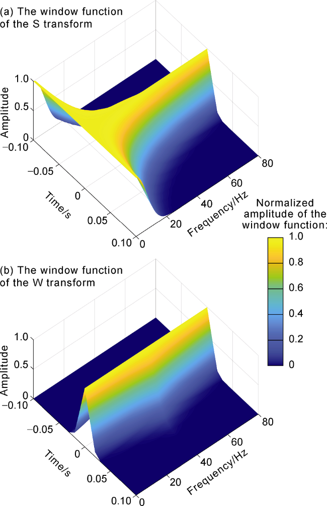
Fig. 1. The comparison between the kernel window of the S transform and that of the W transform. |
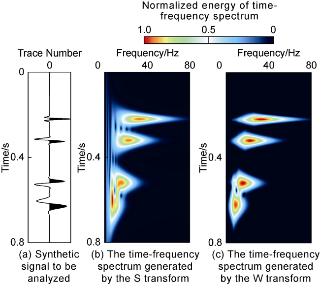
Fig. 2. The comparison between time-frequency spectrum of S transform and W transform. |
The W transform introduces the time-varying instantaneous frequency as an additional parameter, resulting in a time-frequency spectrum with a clear center of gravity of the energy concentration. The Wigner-Ville distribution (WVD) [6], on the other hand, shows the energy distribution in the time-frequency domain and also clearly indicates the time and frequency centroids of wavelets. Therefore, the WVD can serve as a direct benchmark for the W transform, although the WVD is a nonlinear method for time-frequency analysis.
The WVD of a signal $x(t)$ can be expressed as
${{S}_{\text{WVD}}}(t,f)=\int\limits_{-\infty }^{\infty }{z\left( t+\frac{\tau }{2} \right){{z}^{*}}\left( t-\frac{\tau }{2} \right){{\text{e}}^{-\text{i}2\pi f\tau }}\text{d}\tau }$
where $z(t)$ represents the analytic signal of the seismic data, not the original seismic data $x(t)$. Therefore, the WVD can be regarded as the instantaneous autocorrelation spectrum of the seismic analytic signal at any point in time [1]. After Fourier transform, the analytic signal does not have negative frequencies [1], which avoids mutual interference between positive and negative frequency components. Since the WVD is quadratic, it is a nonlinear transform method that inevitably leads to mutual interference between different signal components.
The smoothed pseudo Wigner-Ville distribution (SP- WVD) method [9] effectively suppresses crosstalk. Another relatively complex implementation of WVD is the Matching Pursuit based WVD (MP-WVD) method. By applying the matching pursuit technology [7], the seismic data are decomposed into individual signal components. The time-frequency spectra are then generated individually using the WVD algorithm in Eq. (5), which avoids crosstalk between different signal components.
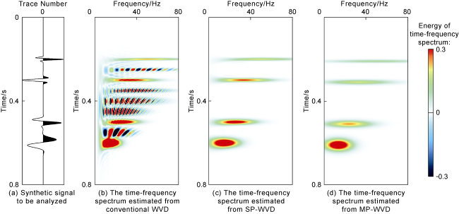
Fig. 3. The time-frequency spectrum estimated with different WVD methods. |
Based on the analysis of Figs. 2 and 3 , the MP-WVD method achieves the highest time-frequency resolution, but with very low computational efficiency. In contrast, the W transform as a representative linear transformation method is much more computationally efficient compared to nonlinear methods such as MP-WVD. However, the time-frequency resolution of the W transform is not as high as that of MP-WVD. Therefore, the standard W transform methods must be further improved.
2. The improved W transforms
As conventional linear time-frequency analysis methods are based on orthogonal time-frequency planes, their application is limited to signals with energy concentrated in harmonic spaces. Given the rapid changes in instantaneous frequency characteristic of strong non-stationary seismic data, conventional time-frequency analysis methods cannot achieve high energy concentration. In recent years, our team has conducted various studies on improved methods based on the W transform suitable for strong non-stationary seismic data. These include harmonic chirp-modulated W transform, fractional order W transform, and linear canonical W transform. Unlike the standard W transform that stretches or compresses window kernel functions, these types of W transforms enhance time-frequency spectrum resolution and energy concentration by altering the angle of the window kernel function or the time-frequency plane. This advancement aims to improve the ability to extract targets such as fluvial channels and thin layers from seismic data.
2.1. Chirp-modulated W transform
To achieve higher energy concentration in time-frequency spectrum of nonstationary seismic data, we propose to introduce a rotation angle into the standard W transform, known as the harmonic variable modulation window W transform. Its mathematical expression is given by [19]:
$\begin{align} & W{{T}_{\text{C}}}\left( \tau,f,c\left( \tau \right) \right)=\frac{\left| {{f}_{0}}\left( \tau \right)+\Delta f \right|}{\sqrt{2\pi }k}\int\limits_{-\infty }^{\infty }{x\left( t \right)w(t-\tau,f;\tau )}\times \\ & \text{ }\ {{\text{e}}^{\text{i}\pi c\left( t-\tau \right){{\left( t-\tau \right)}^{2}}}}{{\text{e}}^{-\text{i}2\pi ft}}\text{d}t, \end{align}$
where the kernel window function is modified to the chirp-modulated kernel window:
${{w}_{\text{c}}}(t,f;\tau )=w(t,f;\tau ){{\text{e}}^{\text{i}\pi {{t}^{2}}c(t)}}$
By introducing the rotation angle, the angle of the time-frequency analysis window can be changed, thereby matching the instantaneous frequency of the seismic data. To select the optimal tuning ratio, the time-frequency plane is first divided into $(N+1)$ regions with the following angle values:
$\theta =\left\{ -\frac{\pi }{2}+\frac{\pi }{N+1},-\frac{\pi }{2}+\frac{2\pi }{N+1},\cdots,-\frac{\pi }{2}+\frac{N\pi }{N+1} \right\}$
The relationship between the chirp rate and the rotational angle is:
$c=-\frac{{{F}_{\text{s}}}}{2{{T}_{\text{s}}}}\tan \theta $
The corresponding chirp-modulated kernel window is given as:
$\begin{align} & W{{T}_{\text{C}}}\left( \tau,f,\theta \right)=\frac{\left| {{f}_{0}}\left( \tau \right)+\Delta f \right|}{\sqrt{2\pi }}\int\limits_{-\infty }^{\infty }{x\left( t \right)w\left( t-\tau,f \right)}\times \\ & \ {{\text{e}}^{-\text{i}\pi \left( {{{F}_{\text{s}}}}/{2{{T}_{\text{s}}}}\; \right){{\left( t-\tau \right)}^{2}}\tan \theta }}{{\text{e}}^{-\text{i}2\pi ft}}\text{d}t. \end{align}$
Since this process involves N successive W transforms, the efficiency of the time-frequency analysis must be improved. In addition, this process inevitably introduces significant artificial noise that potentially reduces the resolution of the time-frequency spectrum. We propose that the chirp rate can be represented as the first derivative of instantaneous frequency with respect to time. This eliminates the artificial noise caused by multiple W transforms while increasing the efficiency of the computation [19].
To improve the efficiency of W transform suffers, the standard W transform should be able to fulfill the requirements of large-scale seismic data processing. Therefore, we are inspired by the method of discrete Fourier transform matrices and represent the W transform as a product of matrix and vector, which can be expressed as follows:
${{W}_{\text{c}}}\left[ :,\text{ }:,\text{ }c\left( t \right) \right]=KX$
whereby matrix K can be calculated on a Graphics Processing Unit (GPU), which considerably reduces the calculation time.
2.2. Fractional-order W transform
The chirp-modulated W transform rotates the analysis window of the W transform in the orthogonal time-frequency plane and achieves optimal resolution and energy concentration by matching the instantaneous frequency of the seismic data. However, for signals with similar frequency components and short time intervals, the effectiveness of this method remains suboptimal. It cannot effectively separate the different seismic signals components and therefore does not achieve the ideal resolution required for time-frequency analysis.
The fractional Fourier transform, a generalization of the Fourier transform, represents time-varying non-stationary signals by rotating the time-frequency plane. To improve the energy concentration and resolution of the W transform for non-stationary seismic data, we combine the fractional Fourier transform with the W transform, and propose the fractional W transform (FrWT) [20]. The α-order fractional W transform of a signal $x(t)$ can be expressed as follows:
$W{{T}_{\text{Fr,}\alpha }}(\tau,u)=\int_{-\infty }^{\infty }{x(t)w\left( \tau -t,u \right)}{{K}_{\alpha }}(t,u)\text{d}t$
where ${{K}_{\alpha }}\left( t,u \right)$ represents the α-order fractional Fourier transform operator and can be expressed as:
${{K}_{\alpha }}\left( t,u \right)=\left\{ \begin{matrix} {{A}_{\alpha }}{{\text{e}}^{\text{i}\pi \left[ {{u}^{2}}\cot (\alpha )-2ut\csc (\alpha )+{{t}^{2}}\cot (\alpha ) \right]}} \\ \delta \left( u-t \right)\text{ } \\ \delta \left( u+t \right)\text{ } \\ \end{matrix} \right.\begin{matrix} \alpha \ne k\pi, \\ \alpha =2k\pi \\ \alpha =\left( 2k+1 \right)\pi \\ \end{matrix}$
${{A}_{\alpha }}=\sqrt{{\left( 1-i\cot \left( \alpha \right) \right)}/{2\pi }\;}$
$w\left( t,u \right)=\frac{{{\left| \left( {{f}_{\text{inst}}}+\Delta u \right) \right|}^{p}}}{\sqrt{2\pi }q}\exp \left( -\frac{{{t}^{2}}{{\left( {{f}_{\text{inst}}}+\Delta u \right)}^{2p}}}{2{{q}^{2}}} \right)$
where $\Delta u=\left| u\csc \left( \alpha \right)-{{f}_{\text{inst}}} \right|$.
Eq. (12) shows that the FrWT can be regarded as a chirp-modulated W transform with the rotation angle ${\theta =\alpha -\pi }/{2}\;$ in the time-frequency plane. FrWT degenerates to the standard W transform, when $\alpha ={\pi }/{2}\;$ and $p=q=1$.
FrWT introduces three additional auxiliary parameters $\left\{ \alpha,\text{ }p,\text{ }q \right\}$ on the basis of the W transform and thus offers more flexibility. The optimization of these auxiliary parameters can be divided into several steps:
(1) Determination of the optimal rotation angle, which is analogous to the chirp-modulated W transform. The best energy concentration is obtained when the optimal rotation angle matches the modulation rate of the signal to be analyzed.
(2) Calculate the fractional W time-frequency spectrum of the signal for different values of p and q.
(3) Evaluate the measure of energy concentration of time-frequency spectra with different fractional orders:
$CM\left( p,q \right)=\frac{1}{\sqrt{\int_{-\infty }^{\infty }{\int_{-\infty }^{\infty }{{{\left| W{{T}_{\text{Fr},\alpha,\text{ }(p,q)}}\left( \tau,u \right) \right|}^{2}}\text{d}\tau \text{d}u}}}}$
(4) Define the optimal parameters p and q as:
${{\left( p,q \right)}_{\text{opt}}}=\underset{\left( p,q \right)}{\mathop{\max }}\,\left| CM\left( p,q \right) \right|$
Although the FrWT requires multiple W transforms, its time complexity is relatively low due to the use of Eq. (11), making it suitable for time-frequency analysis of large- scale seismic data. The fractional W transform combines the properties of the standard W transform and the fractional Fourier transform. It retains the high resolution in the low-frequency range unchanged and improves the resolution of the time-frequency spectrum of non-stationary seismic data by varying the order of the fractional W transform.
2.3. Linear canonical W transform
We further generalize the rotation of the time-frequency plane in the above time-frequency domain by combining the W transform with the linear canonical transform and proposing the method of linear canonical W transform [23]. The linear canonical transform is a more general transform than the rotation relation and is a type of affine transform [22]. Affine transforms are commonly used in applications such as image processing and optical propagation. By introducing three free parameters, the linear canonical transform also provides a more generalized representation compared to the fractional Fourier transform.
Linear canonical transform can be mathematically expressed as:
${{X}_{M}}\left( u \right)={{L}_{M}}\left( x(t) \right)\left( u \right)=\left\{ \begin{matrix} \int_{-\infty }^{\infty }{x(t)}{{K}_{M}}\left( t,u \right)\text{d}t\text{ }B\ne 0 \\ \sqrt{D}{{\text{e}}^{\text{i}{CD{{u}^{2}}}/{2}\;}}x\left( Du \right)\text{ }B=0 \\ \end{matrix} \right.$
where ${{K}_{M}}\left( t,u \right)$ represents the kernel of the linear canonical transform, mathematically expressed as:
${{K}_{M}}\left( t,u \right)=\frac{1}{\sqrt{2\pi Bi}}{{\text{e}}^{i\ {\left( A{{t}^{2}}-2ut+D{{u}^{2}} \right)}/{\left( 2B \right)}\;}}$
From Eqs. (18) and (19), it can be seen that compared to the standard Fourier transform, the linear canonical transform adds 4 parameters A, B, C and D. These 4 parameters can form a matrix:
$M=\left( \begin{matrix} A & B \\ C & D \\ \end{matrix} \right)=[A,B,C,D]$
The matrix satisfies the symplectic condition,$AD-BC=1$. This condition ensures that the entire support region of the signal in the time-frequency plane doesn’t change, and the linear canonical transform has perfect reconstruction capability. Eqs. (18) and (19) show that in practical calculations the presence of parameter C is only taken into account if $B=0$. When $B=0$, linear canonical transform degenerates to a simple modulation transform.
By adjusting the parameters of the matrix, the linear canonical transform can degenerate into various transforms, including the Fresnel transform, the Fourier transform and the fractional Fourier transform. Therefore, the linear canonical transform offers greater flexibility than the fractional Fourier transform and a wider range of applications.
If the linear canonical transform is combined with the W transform, the linear canonical W transform can be represented as follows:
$\begin{align} & WT_{\text{LC}}^{\text{M}}\left( \tau,u \right)=\int\limits_{-\infty }^{\infty }{x(t)w\left( \tau -t,u \right){{\text{e}}^{\text{i}\pi {(A{{t}^{2}}-D{{\tau }^{2}})}/{(2B)}\;}}{{\text{e}}^{-\text{i}2\pi ({u}/{B}\;)t}}\text{d}t} \\ & =\int\limits_{-\infty }^{\infty }{x(t){{w}_{M}}\left( \tau -t,u \right){{\text{e}}^{-\text{i}2\pi ({u}/{B}\;)t}}\text{d}t} \end{align}$
where
$w\left( t,u,\tau \right)=\frac{{{\left| \left( {{f}_{0}}\left( \tau \right)+\Delta u \right) \right|}^{p}}}{\sqrt{2\pi }q}{{\operatorname{e}}^{-{{{t}^{2}}{{\left( {{f}_{0}}\left( \tau \right)+\Delta u \right)}^{2p}}}/{\left( 2{{q}^{2}} \right)}\;}}$
$\Delta u=\left| {u}/{B}\;-{{f}_{0}}\left( \tau \right) \right|$
The Linear Canonical W transform can apply various linear transformations to the support domain of conventional time-frequency algorithms, including translation, scaling and shearing. From Eq. (21), it can be seen that when the matrix M takes the form $M=[\cos \alpha,$ $\sin \alpha,\text{ }-\sin \alpha,\text{ }\cos \alpha ]$, the Linear Canonical W transform degenerates into a $\alpha \text{-order}$ fractional W transform; and into a standard W transform when $M=[\text{ }0]$. The support domains of the various W transforms are shown in Fig. 4 . It can be seen that the transition from the W transform to the fractional W transform and then to the linear canonical W transform represents a process of continuous generalization that increases the flexibility of the W transform.
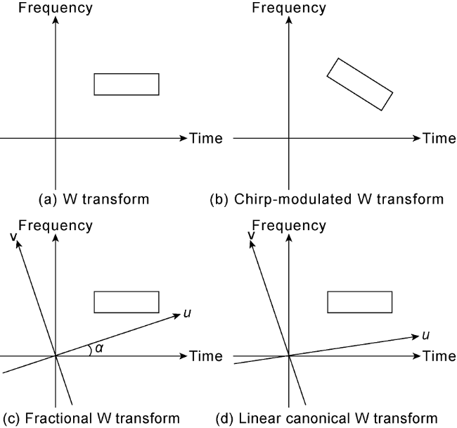
Fig. 4. Support regions of different W transforms. |
The parameter optimization of the Linear Canonical W transform is similar to that of the fractional W transform, with the difference that in the linear canonical transform, the highest energy concentration in the time-frequency spectrum is only achieved if the value of ${A}/{B}\;$ is the negative reciprocal of the chirp rate of the signal. The introduction of the Linear Canonical W transform not only offers promising applications in the identification of thin-layer hydrocarbon reservoirs in non-stationary seismic data, but also expands the significance of the W transform in fields such as optics and image processing.
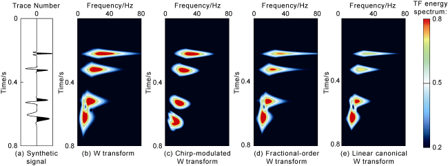
Fig. 5. Time-frequency spectra estimated by different W transforms. |
3. Application examples
This paper demonstrates the practical application effects of three W transforms. First, field seismic data were extracted to verify the application of the W transform in the seismic detection of fluvial sand bodies. Numerous ancient river channels can be identified in the first case (Fig. 6a ), although the channel boundaries are not clear and continuity needs to be improved. Fig. 6b shows the time slice along the layered disc, while Fig. 6c and 6d show the corresponding SP-WVD time-frequency spectrum along the layered slice and the standard W transform time-frequency spectrum along the layered slices with a frequency of 40 Hz. The time- frequency spectrum slices of the W transform show clearer fluvial channel edges and accurately represent the channel orientations. Therefore, the W transform time-frequency spectrum can effectively delineate the boundaries of underground reservoirs.

Fig. 6. Fluvial channel detection by SP-WVD and W transform. |
The second example confirms the effectiveness of the W transform in detecting karst caves. Fig. 7a shows a seismic profile extracted from actual 3D seismic data volume with clear "bead-like" seismic reflections. However, the time domain seismic profile does not indicate whether these "bead-like" seismic reflections are caused by karst caves. We use the SP-WVD method, the MP-WVD method and the standard W transform method to perform a time-frequency analysis of this profile and extract frequency slices corresponding to 40 Hz.
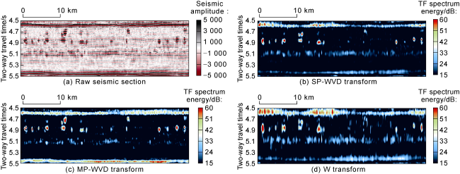
Fig. 7. Karst caves detection by SP-WVD, MP-WVD and W transform. |
The above three methods effectively decompose the original seismic profile into seismic frequency spectrum slices with different frequencies, thus facilitating the detection and identification of karst caves in seismic data. However, unlike conventional time-frequency analysis methods based on orthogonal windows, the W transform also has a high resolution in the low-frequency range. This capability helps to reveal the “low-frequency shadows” in seismic data and thus effectively guide the drilling process.
The third example confirms the effectiveness of different W transform methods in detecting multiphase fluvial channels. Fig. 8a shows an isochronous 3D seismic slice, which indicates the development of several fluvial channels. However, the isochronous profile of the seismic data shows poor resolution, unclear channel boundaries and unclear channel distribution. Fig. 8b -8e show RGB fused time-frequency spectra obtained with standard W transform, chirp-modulated W transform, fractional W transform and linear canonical W transform.

Fig. 8. Fluvial channel detection by W transform, chirp-modulated W transform, fractional W transform and linear canonical W transform. |
From the images of the RGB fused slices, it can be seen that the region has several fluvial channels and that the boundaries in the RGB fused slices are more clearly visible compared to the seismic isochronous slices. The time-frequency spectra obtained from the fractional W transform and linear canonical W transform show clearer and less disturbed fluvial channels, which effectively improves the resolution of seismic detection of ancient fluvial channels.
4. Conclusions
This paper provides a comprehensive overview of the development of the W transform method for time-frequency analysis and its improvement. The recently proposed W transform is a typical linear time-frequency analysis method. Linear time-frequency analysis is performed with a convolution between seismic signals and specific window functions and provides clear theoretical foundations and simple calculations. However, it often fails to achieve high resolution and energy concentration in both time and frequency domains simultaneously, mainly due to poor resolution in the low-frequency range. To address the problem of poor resolution in the low-frequency range in linear time-frequency analysis methods, we have recently introduced the W transform. By including the instantaneous frequency of the seismic data as one of its parameters, the W transform constructs analysis windows symmetrically around the instantaneous frequency of the seismic data. This approach has improved the resolution of linear time-frequency analysis methods in the low-frequency range.
This paper contrasts the W transform with the Wigner-Ville distribution method (WVD). The WVD method is a representative of nonlinear time-frequency analysis methods, and its nonlinear nature often leads to problems with crosstalk between different signal components in seismic data, which significantly affects the effectiveness of time-frequency analysis. However, the time-frequency energy distribution revealed by the WVD method clearly indicates the time and frequency centroids of seismic wavelets, which serves as a direct benchmark for the W transform. In the W transform, the introduction of the instantaneous frequency as a parameter corresponding to any time position ensures that the displayed time-frequency spectrum also shows a clear focus of the energy centers.
In this manuscript we deal in detail with various improvements of the W transform with the aim of continuously generalizing its methods. These improvements utilize linear transformations such as scaling, rotation and shearing to improve the resolution and energy concentration of the W transform time-frequency spectra. These methods are particularly applicable to non-stationary seismic data, especially in regions rich in oil and gas reservoirs. By applying different degrees of rotation transformation to the time-frequency axis, the energy concentration of the time-frequency spectra can be improved. These approaches have proven to be very useful in practice for reservoir characterization, exploration of ancient fluvial channels and other related fields.
Nomenclature
{A, B, C, D}—parameters in linear canonical transform;
$c(t)$—chirp rate, Hz/s;
${{A}_{\alpha }}$—the normalized factor of fractional Flourier transform;
CM—energy focus, dimensionless;
f—frequency, Hz;
${{f}_{0}}\left( t \right)$—the instantaneous frequency at t, Hz;
${{f}_{0}}\left( \tau \right)$—the instantaneous frequency at analysis window, Hz;
${{f}_{\text{inst}}}$—instantaneous frequency, Hz;
Fs—frequency interval, Hz;
i—imaginary unit;
k—the scale factor in time-frequency analysis, dimensionless;
K—the discrete W transform matrix at different frequencies;
${{L}_{\text{M}}}$—the operator of linear canonical transform;
${{K}_{\text{M}}}\left( t,u \right)$—the kernel function of linear canonical W transform;
${{K}_{\alpha }}\left( t,u \right)$—the operator of α-order fractional W transform;
M—a matrix formed by parameters {A, B, C, D} in linear canonical transform;
N—the number of time-frequency sections in the time-frequency plane in chirp-modulated W transform;
$\{p,\text{ }q\}$—two auxiliary parameters controlling analysis window length, dimensionless;
${{S}_{\text{SP-WVD}}}(t,f)$—the time-frequency spectrum estimated from SP-WVD, dimensionless;
${{S}_{\text{WVD}}}\left( t,f \right)$—the time-frequency spectrum estimated from WVD, dimensionless;
$ST\left( t,f \right)$—the time-frequency spectrum estimated from S transform, dimensionless;
t—time, s;
Ts—time sampling interval, s;
u—auxiliary parameter, dimensionless;
$w\left( t \right)$—the window kernel function in W transform;
$w(t,f;\tau )$—the window function in W transform;
${{w}_{c}}(t,f;\tau )$—the window function in chirp-modulated W transform;
${{w}_{M}}\left( \tau,u \right)$—the window function in linear canonical W transform;
${{W}_{C}}\left[ :,:,c\left( t \right) \right]$—the time-frequency spectrum in chirp-modulated W transform;
$WT\left( t,f \right)$—the time-frequency spectrum estimated from W transform, dimensionless, dimensionless;
$W{{T}_{\text{C}}}\left( \tau,f,c\left( \tau \right) \right)$—the time-frequency spectrum estimated from chirp-modulated W transform, dimensionless;
$T_{\text{Fr,}\alpha }^{{}}(\tau,u)$—the time-frequency spectrum estimated from fractional-order W transform, dimensionless;
$WT_{\text{LC}}^{\text{M}}(\tau,u)$—the time-frequency spectrum estimated from linear canonical W transform, dimensionless;
$c(t)$$x\left( t \right)$—seismic signal;
X—the seismic signal vector;
${{X}_{\text{M}}}$—the frequency spectrum from linear canonical W transform, dB;
$z\left( t \right)$—the analytical form of seismic signal;
α—the order of fractional W transform;
τ—the time of analysis function, s;
π—ratio of circumference to diameter;
*—convolution;
ϕ—the phase of a wavelet;
θ—the rotational angle of the time-frequency plane;
δ—unit step function;
$\Delta f$—the absolute difference between the dominant frequency and the frequency to be analyzed, Hz;
$\Delta u$—the absolute difference between the dominant frequency and the frequency to be analyzed in different transforms, Hz.