

Introduction
Shale oil and gas plays are subsets of what the U.S. Geological Survey designates as “continuous resources” [1]. These types of reservoirs do not occur in discrete traps or form through hydrocarbon migration, but rather are regionally extensive accumulations of hydrocarbons, generally in rocks with relatively low matrix permeability [1-2]. In the strictest sense, a shale play is one where a shale interval acts as both the source rock and the reservoir [3], but in practice, a variety of rock types contribute to production in shale plays.
Although the prominence of shale oil and gas production is relatively recent, there has been production from shale reservoirs in the United States periodically for almost 200 years. The first commercial natural gas well in the U.S. was drilled in fractured Late Devonian shales near the town of Fredonia in western New York in 1825 [4]. In 1863, commercial gas production in Kentucky began from fractured Devonian shales, with production from this play continuing into the 1990s [5].
Techniques used to produce oil and gas from these wells are also not entirely new. The first horizontal well was drilled in Texas in 1929 [6]. The first fracture stimulation of a gas well, using 3.6 kg (8 pounds) of gunpowder, took place in western New York in 1857 [4] and nitroglycerin was used for fracturing in oil wells as early as the 1860s [7]. Hydraulic fracturing was developed by Stanolind Oil and first used to stimulate a limestone reservoir in 1947 [7]. In 1949, the hydraulic fracturing technology was patented and licensed to Halliburton [7].
Shale oil production began with the discovery of the Antelope Field in the Williston Basin of North Dakota in 1953 [6]. While some production was from a localized sand reservoir, there was also production from fractured Mississippian shales of the Upper Member of the Bakken Formation [8]. Sporadic drilling continued in the Bakken in the 1960s and into the early 1970s.
The late 1970s and 1980s saw a new focus on the potential of shale oil and gas production. Following the U.S. energy shortages of the 1970s, the U.S. government sponsored researches on improving the understanding and production of gas-bearing shales, particularly in the eastern U.S. [9]. Collaboration between the U.S. Department of Energy, the Gas Research Institute, and operating companies in the late 1970s and 1980s included experiments with horizontal drilling and new methods of hydraulic fracturing [10]. Horizontal drilling became more commercially viable with the introduction of improved downhole motors [6].
In the late 1970s, Mitchell Energy Corporation (MEC), which owned a network of gas infrastructure in North Texas, was looking for new sources of gas to replace declining production from conventional fields in the Pennsylvanian section of the Fort Worth Basin [11]. There had been consistent gas shows in the Late Mississippian Barnett shale in wells targeting deeper Ordovician carbonates, so in 1981, MEC drilled and hydraulically fractured the first well targeting the Barnett shale [11]. MEC drilled 100 wells between 1981 and 1990, with massive gel-based hydraulic fracture treatments starting in 1985 [11-12].
The 1980’s also saw a renewed focus on oil production from Bakken shales with experiments applying hydraulic fracturing in vertical wells [8,13]. In 1987, Meridian Oil completed the first horizontal well in the Bakken Formation in an attempt to encounter additional vertical fractures within the shale reservoir [13]. While horizontal wells did improve performance over vertical wells, drilling in the Bakken remained marginally economic [13-14].
The period from 1995 to 2002 was the turning point in the development of shale oil and gas as commercial resources. In 1995, an exploration geologist determined that there was a high-porosity fractured dolomite in the Middle Member of the Bakken Formation in the Williston Basin of Montana, which might act as a reservoir for the oil generated in the Upper Bakken shales [13,15]. In 1996-1997, several vertical wells were drilled to test the dolomite interval, leading to discovery of the Elm Coulee Field [15]. Meanwhile, in 1998, MEC changed its approach to well stimulation in the Barnett shale, switching from gel-based to water-based fracturing fluid, which greatly reduced fracturing costs [11]. In 2000, the first horizontal well was drilled and fracture-stimulated in the Elm Coulee Field [13,15]. In 2002, Devon Energy, which had bought MEC, experimented with seven horizontal wells in the Barnett, which both improved production and reduced the risks of fracturing into other formations which may be water-bearing [11].
The development of drilling and completion technologies and practices that allowed for commercial development of shale oil and gas was a major breakthrough for hydrocarbon production in the U.S., with these plays becoming increasingly important over time. Since 2007 to 2023, production from shale oil and gas reservoirs has increased from 11.2×10⁴ t/d of oil equivalent to over 300.0×10⁴ t/d of oil equivalent [16]. Looked at in terms of the total U.S. production, the contribution from shale plays increased from 5% in 2007 to over 60% in 2023 (Fig. 1 ).
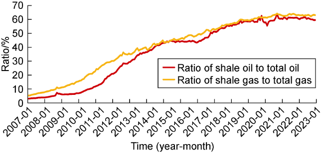
Fig. 1. U.S. shale oil and gas production as a percentage of total U.S. oil and gas production from 2007 to 2023 [16]. |
The U.S. Energy Information Administration (EIA) has identified a significant number of existing and potential shale plays within the United States [16]. In this paper, we will focus on those plays that have seen significant development using horizontal drilling combined with hydraulic fracturing (Fig. 2 ). Based on the analysis of geological evolution and features, development status, quantity of resource and production variation of major basins, new trends of U.S. shale oil and gas development technologies were pointed out.
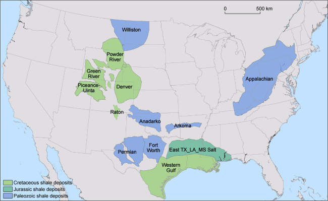
Fig. 2. Distribution of basins hosting major shale plays in U.S. [16]. |
1. Geologic development of shale basins
Productive shales within major basins range in age from Mid-Ordovician to Late Cretaceous: Middle Ordovician, Middle to Late Devonian, Early Carboniferous (Middle to Late Mississippian), Early Permian, and Late Jurassic and Late Cretaceous (Cenomanian-Turonian) (Fig. 3 ). Some current basin outlines are a result of tectonic events that occurred after deposition of the productive shales that occur within the basin. In these instances, the productive shales may be partially exposed along or even eroded from the basin margins. For this reason, their first part of the discussion will focus on the geological evolution characteristics of these basins developed productive shales.
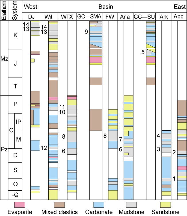
Fig. 3. Simplified stratigraphic columns for major U.S. basins that host shale plays. App-Appalachian Basin [26]; Ark- Arkoma Basin (Arkansas section shown) [27]; GC-SU-Gulf Coast Sabine Uplift [28-29]; Ana-Anadarko Basin [30]; FW- Fort Worth Basin [31]; GC-SMA-Gulf Coast San Marcos Arch [28-29]; WTX-West Texas Basin (Permian Basin) [32]; Wil -Williston Basin [33]; DJ-Denver-Julesberg basins [34]. List of shale plays (* indicates not currently productive): 1-Utica/Point Pleasant, 2-Marcellus, 3-Chattanooga*, 4-Fayetteville, 5-Haynesville/Bossier, 6-Woodford, 7-Caney*, 8-Barnett, 9-Eagle Ford, 10-Wolfcamp, 11-Bone Springs/ Spraberry, 12-Bakken, 13-Niobrara, 14-Pierre/Mancos*. |
1.1. Paleozoic basins
Other than the Williston Basin, the U.S. basins that host Paleozoic shale plays share a similar geologic history related to the location on the margins of Laurentia between the breakup of Rodinia and the formation of Pangea.
Rifting associated with the breakup of Rodina occurred during the late Neoproterozoic to the Cambrian, followed by an initial pulse of clastic sedimentation [17]. In the Early Ordovician, sea-level rise led to development of a carbonate bank that covered most of the contiguous United States [18]. During the Middle Ordovician, a complex island arc terrane collided with the margin of Laurentia in what is now the northeastern U.S., resulting in the Taconic Orogeny [17]. The Utica shale, the oldest of the productive shales discussed here, was deposited in the foreland basin associated with this orogenic event (Appalachian Basin) [17,19⇓ -21] (Fig. 4a ). At this time, the Williston Basin, an intracratonic basin unrelated to the orogeny to the east, also develops as a distinct feature [22].
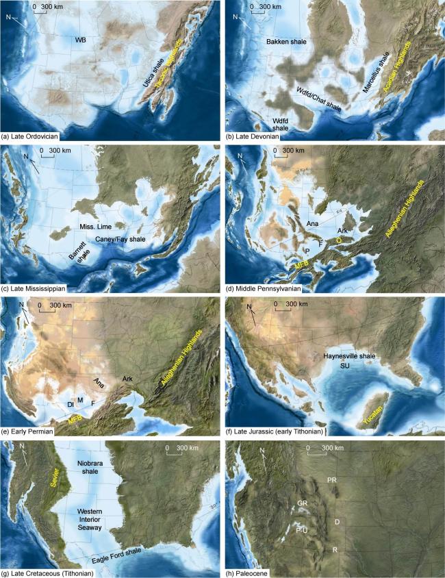
Fig. 4. Paleogeographic maps of North America during deposition of key productive shale intervals [55⇓⇓⇓⇓⇓⇓⇓⇓-64]. WB—Williston Basin; Wdfd/Chat—Woodford/Chattanooga; Fay—Fayetteville Chat; P—Permian Basin; F—Fort Worth Mountain; Ana—Anadarko Basin; Ark—Arkoma Basin; MFB—Marathon Fold Belt; O—Ouachita Mountains; Dl—Delaware Basin; M—Midland Basin; SU—Sabine Uplift; PR—Powder River Basin; GR—Green River Basin; P-U—Piceance-Uinta Basin; D—Denver Basin; R—Raton Basin. |
A second orogenic event related to development of the Appalachian Mountains and foreland basins took place in the Middle Devonian to Early Mississippian as the Amorica microcontinent was accreted onto Laurentia [17,20,23]. The resulting foreland basin was near-coincident with the earlier Taconic foreland basin (Fig. 4b ) and its sedimentary fillings include the Marcellus shale and other Devonian black shales of the Appalachian Basin [4,8,23]. On the southwestern margin of Laurentia, widespread transgression led to deposition of black shales (the Woodford and Chattanooga shales) in a passive margin setting with organic productivity increased by upwelling [24-25]. During this same period, the Bakken Shale was also deposited as a response to transgression in the Williston Basin [22]. This Middle to Late Devonian period essentially has simultaneous deposition of productive shales in a foreland basin, along a passive margin, and within an intracratonic basin.
In the Early to Middle Mississippian (Early Carboniferous) (Fig. 4c ), deposition in the Williston Basin switched to platform carbonates [22]. In the Appalachian Basin, shallow water sedimentation dominated, although there were also periods of arching and erosion periodically within this period [19]. Neither area has developed productive shales of this age. Along the southwestern passive margin, continued transgression led to drowning of previously uplifted areas and deposition of a sequence of landward platform carbonates and seaward shales, including the Barnett, Caney and Fayetteville shales [23⇓-25,35].
The Late Mississippian to Permian saw multiple tectonic events associated with the collision between Gondwana and Laurentia that resulted in the assembly of Pangea. One impact of this was the development of a series of thin-skinned fold and thrust belts along the southern margin of Laurentia: the Alleghenian, Ouachita, and Marathon orogens [36-37] (Fig. 4d ). The classic fold-thrust sequences of the Valley-and-Ridge province of the Appalachian Mountains incorporated sediments from the older Appalachian foreland basins [36]. The Arkoma and Fort Worth basins (Fig. 4d ) developed as foreland basins to the Ouachita orogenic belt [25,35⇓⇓ -38]. This collision also produced a complex series of basement-cored uplifts known as the Ancestral Rocky Mountains (ARM) that are widely distributed across central and western North America [39⇓-41]. Shale basins associated with Ancestral Rockies deformation include the Anadarko and Ardmore basins of Oklahoma, and the Permian Basin of West Texas and New Mexico [39⇓-41]. The segmentation of the Permian Basin area into the Delaware and Midland basins had yet to develop, as ARM deformation began earlier in Oklahoma than in West Texas [39].
Pennsylvanian sedimentation in both the foreland basins and the ARM basins was complex, with coarse clastic sediments shed from the associated uplifts interspersed with shallow water carbonates [26,31,42⇓ -44]. Part of the complexity is produced by sea level changes driven by pulses of glaciation during this time period [42]. Meanwhile, sedimentation in the intracratonic Williston Basin was dominated by terrestrial to shallow marine sediments and evaporites [31]. No productive shale plays of this age have been discovered, likely due to increased terrigenous input from uplifted areas.
ARM deformation was active from the Middle Pennsylvanian (Atokan) to Early Permian (Wolfcampian) [39,41]. In the Permian Basin, this deformation produced a series of central uplifts (the Central Basin Platform or CBP) with the deeper Delaware Basin to the west, and shallower Midland Basin to the east [42] (Fig. 4e ). Throughout the Pennsylvanian to the Early Permian, there was a mixed system of carbonates and clastics with platform carbonates on the uplifted CBP and shelves, and basinal carbonates and shales in the subsiding basins [23,42]. By Leonardian (later Early Permian) time, deformation had ceased and sedimentation patterns in the basins were primarily driven by sea level changes, with carbonate- and mud-rich facies deposited during highstands and detrital silts and sands during lowstands [23,45 -46]. It is the basinal facies of the Wolfcampian and Leonardian intervals that have been the basis for most shale oil and gas produced from the Midland and Delaware basins.
1.2. Mesozoic basins
If the development of the Paleozoic shale basins was generally centered on the assembly of Pangea, the development of the Mesozoic shale basins begins with the breakup of Pangea and the formation of the Gulf of Mexico. During the Late Triassic and Early Jurassic, a rift system formed that began to separate the southern margin of the North American plate from the South American and African plates with the northern part of the basin consisting of a series of horsts and grabens [47-48]. By the late Middle Jurassic (Callovian), periodic incursions of seawater led to widespread evaporite deposition [47]. By the early Late Jurassic (Oxfordian), rifting had ceased following a period of oceanic crust emplacement as the Yucatan block moved away from the North American plate [48] (Fig. 4f ). Following this there was a period of marine transgression that continued into the Early Cretaceous [48-49]. During the early stages of this transgression, the Mid-Late Jurassic (Kimmeridgian) Haynesville Shale (Fig. 4 ) was deposited on the crest and eastern flank of the Sabine uplift, one of the isolated horst blocks [49-50]. Both lithology and terminology in the Kimmeridgian section are variable, and the shale facies is sometimes referred to as the Bossier Shale [49]. To the east and west of the Sabine Uplift area, the Haynesville section is dominated by carbonates [49].
The early Late Cretaceous saw the deposition of the youngest shale plays, the Eagle Ford Group and the Niobrara Formation (Fig. 4g ). The Eagle Ford Group was deposited along the Gulf of Mexico margin above an older carbonate platform in the late Cenomanian to Turonian [51].organic-rich marls and associated limestones within the Eagle Ford are largely restricted to the area west of the San Marcos Arch, an intermittently-active anticline of uncertain origin [51⇓⇓-54]. To the east of the arch, the influence of the Woodbine and Harris Deltas results in the Eagle Ford being more clay-rich [51,53].
Along the western margin of North America, plate convergence and accretion of various terranes had been ongoing since the Late Devonian [55]. By Cenomanian-Turonian time, a thin-skinned thrust belt (Sevier Orogeny) had developed well inboard of the continental margin [55-56]. A combination of global transgression and downwarping of the Sevier foreland basin, led to flooding of the interior of North America to form the Western Interior Seaway [57]. The Niobrara Formation and correlative stratigraphic units were deposited over much of the seaway during Coniacian to early Campanian time [58-59] (Fig. 4g ), but final basin development was not yet complete. Continued crustal shortening in the Late Cretaceous to Eocene (Laramide Orogeny) produced basement cored uplifts and associated basins, segmenting the formerly continuous Niobrara Formation [55,60⇓ -62] (Fig. 4h ).
2. Play descriptions
In this section, we present a brief description of the major shale plays in U.S., highlighting the history of the play, some characteristics of production and key components of the geology. Table 1 lists basic information about distribution area, thickness, porosity, clay content and TOC of major shale strata in U.S.
Table 1. Comparison of geologic properties between shale plays in U.S. |
| Strata | Area/km2 | Depth/m | Thickness/m | Porosity/% | Clay content/ % | TOC/% | Lithofacies | |
|---|---|---|---|---|---|---|---|---|
| Series | Formation | |||||||
| Upper Cretaceous | Niobrara | Denver-Julesberg basins: 15 680*, Powder river basin: 10 734* | Powder river basin: 610- 2 134 [63] | Powder river basin: 46-198 [63] | Powder river basin: 3.0- 8.0 [64] | 20-30 [63] | Denver-Julesberg basins: 0.5-8.0, avg. 3.2 [64] Powder river basin: 0.90-3.24 [63] | Interbedded chalks and marl, sandstones locally to the west, grading into shale and siltstone in center of basin [64] |
| Eagle Ford | 35 584 [65] | 232- 4 893, avg. 2 583 [65] | 8-78, avg. 37 [65] | avg. 6.6 [65] | 14-20 [65] | 0.82-4.94, avg. 2.62 [65] | Organic-rich marls, planktonic foraminferal packstones and grainstones, increasing clay east of the San Marcos Arc [51] | |
| Upper Jurassic | Haynesville | 14 747 [65] | 3 102- 4 939, avg. 3 589 [65] | 0-117, avg. 62 [65] | avg. 6.7 [65] | 10-50 [65] | 0.7-6.2 [50] | Bioturbated calcareous mudstone, laminated calcareous mudstone, silty peloidal siliceous mudstone, unlaminated siliceous organic-rich mudstone [50] |
| Lower Permian | Midland Wolfcamp | 39 648 [65] | 210-2 133, avg. 1 465 [65] | 210-1 302, avg. 554 [65] | avg. 7.6 [65] | 26 [65] | 0.5-6.4, avg. 2.4 [65] | Silicieous mudrock, calcareous mudrock, muddy bioclast-lithoclast floatstone, skeletal wackestone/packstone [65] |
| Delaware Wolfcamp | 32 864 [65] | 170-2 867, avg. 1 942 [65] | 38-2 989, avg. 865 [65] | avg. 7.6 [65] | 21 [65] | 0.5-7.3, avg. 2.3 [65] | Argillaceous mudrock, siliceous mudrock, muddy bioclast-lithoclast floatstone, skeletal wackestone/packstone, muddy floatstone [65] | |
| Upper Mississippian | Fayetteville | 6 032 [65] | 80-2 401, avg. 886 [65] | 18-215, avg. 83 [65] | avg. 6.3 [65] | 29- 32 [66] | 0.1-10.8, avg. 4.07 [65] | Black to gray shale, higher organic content in lower Fayetteville, local sandstone separating upper and lower shales [67] |
| Barnett | 21 111 [65] | 799-2 484, avg. 1 638 [65] | 18-28, avg. 87 [65] | avg. 5.6 [65] | 27 [68] | 2.0-6.0 [68]; 0.36-9.66, avg. 3.1 [69]; 3.3-4.5 [43] | Laminated siliceous mudstone, laminated argillaceous lime mudstone, skeletal, argillaceous lime packstone [70] | |
| Upper Devonian-Lower Mississippian | Bakken | 44 853 [65] | 1 376- 2 737, avg. 2 286 [65] | 0-24, avg. 11 [65] | avg. 5.9 [65] | 20-30 [71] | 1.79-20.20, avg. 2.62 [65] | Siliceous organic-rich mudrocks, wackestones, calcareous sandstones and siltstones, dolostones, siltstones, and dolomitic mudrocks [65] |
| Upper Devonian | Woodford | 35 715* | Avg. 2 610 [72] | Avg. 75 [72] | 3.0- 6.8 [73] | 15-38 [72] | 5.0-6.5 [72] | Clayey mudrock, clayey siliceous mudrock, dolomitic clayey mudrock, siliceous mudrock, Increasing chert interbeds to south [72] |
| Middle Devonian | Marcellus | 46 648 [65] | 95-2 239, avg. 1 325 [65] | 3-178, avg. 39 [65] | avg. 7.4 [65] | 0-65 [65] | 1-10 [68]; 1.4-4.3 [74]; 3.87-11.25 [75]; 0.17-7.22, avg. 2.11 [76] | Coarse-grain calcareous mudstone, skeletal wackestone-packstone limestone, calcitic carbonaceous medium-grain mudstone, silicieous carbonaceous fine-grain mudstone, and argillaceous coarse-grain mudstone [77] |
| Middle Ordovician | Utica/ Point Pleasant | 63 772* | 933-3 773, avg. 2 348 [78] | 17-75, avg. 46 [78] | 3.2- 6.5 [79] | 32-49 [77] | Utica: 1.0-3.5; Upper Pt Pleasant: less than 1; Lower Pt Pleasant: 3-8, avg. 4-5 [80] | Utica: calcareous shale (10%-60% calcite); Upper Pt Pleasant: organic poor shale with thin carbonates; Lower Pt Pleasant: organic-rich calcareous shale (40%-60% carbonate) [80] |
Note that values with * estimated from producing well distribution range. |
2.1. Paleozoic plays
2.1.1. Appalachian Basin
The Utica shale play is present primarily in Ohio, but extends into western and northern Pennsylvania, as well as West Virginia. The play extends into New York, but a ban on hydraulic fracturing in the state has prevented development there. Utica production in eastern Ohio, West Virginia, and Pennsylvania is dominated by shale gas, but oil production increases to the west in Ohio and parts of northwestern Pennsylvania (Fig. 5a ). Initial production took place in Quebec, Canada from two vertical wells drilled by Forest Oil in 2008 [81]. Talisman Energy began operations in Quebec in 2009, but a moratorium on hydraulic fracturing in 2012 by the province ended this phase of exploration [81]. Chesapeake Energy completed four wells in the Utica in Ohio in 2011, including three in the oil-rich regions of the play. The Utica shale play covers an area of about 64 000 km2, and has produced from almost 3 300 wells [82].
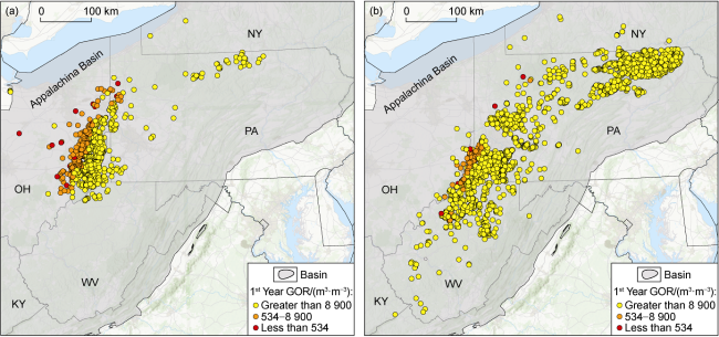
Fig. 5. Production data for Utica shale wells (a) and Marcellus Shale wells (b) [82]. NY—New York, PA—Pennsylvania, OH—Ohio, WV—West Virginia, KY—Kentucky. |
The Utica is a hybrid play that includes the calcareous shales of the Utica Formation and the interbedded limestones and shales of the Point Pleasant Formation [78,80]. The Point Pleasant tends to have higher content of total organic carbon (TOC) than the Utica [80], and the combination of this with the higher carbonate content may explain why most wells target the Point Pleasant [78]. The Utica shale reaches a thickness of 60-90 m in eastern Ohio and northwestern Pennsylvania, thinning to less than 15 m in southern Ohio, while Point Pleasant thickness is in excess of 60 m in central Pennsylvania and thins to less than 6 m in eastern Kentucky [80].
Exploration of Middle Devonian Marcellus shale play began when Range Resources drilled a well with an Early Silurian target in 2003 and encountered significant gas shows in the Marcellus [83]. Following up using techniques developed in the Bakken, Range began producing gas commercially from the Marcellus in 2007 [84]. The Marcellus play covers an area of 140 000 km2 and has an average thickness of 30 m [85]. Production from the Marcellus is primarily in Pennsylvania, but extends into West Virginia, and to a lesser extent in Ohio (Fig. 5 ). Production is dominated by dry gas, but some condensate is produced towards the western edges of the play. Almost 15 000 wells have been put into production from the Marcellus since 2003. For most of its extent, the Marcellus consists of two black shale intervals separated by a sequence of mixed limestone and shale [65,86]. This sequence can reach a thickness where it acts as a barrier to hydraulic fracturing, which can be developed by stacked horizontal wells [65].
2.1.2. Woodford shale and Chattanooga shale
The Late Devonian Woodford shale is a major shale play in Oklahoma and is also attracting interest in the Permian Basin of Texas (Fig. 6 ). Most production is from basins that formed in response to collision of Laurentia and Gondwana (Anadarko, Arkoma, Ardmore/Marietta, Permian), but there is also production from the Cherokee Platform, part of the southern Laurentian passive margin that was not impacted by the collision [87-88]. The Chattanooga shale of the Arkansas portion of the Arkoma Basin appears to have only been tested by one well [82] (Fig. 6 ). While the Chattanooga may have some potential, it is generally too thin or too deeply buried to be prospective [34]. Woodford production in the Arkoma Basin is dominated by gas, but the other Oklahoma basins are more oil-prone (Fig. 6 ). The limited data from the Permian Basin suggest that the western edge of the Delaware Basin tends to be more gas-prone, with oil towards the Central Basin Platform and the Midland Basin.
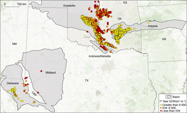
Fig. 6. Production data for Woodford Shale and Chattanooga Shale (Arkansas) [82]. CBP—Central Basin Platform, KS—Kansas, OK—Oklahoma, AR—Arkansas, TX—Texas, NM—New Mexico. |
The first Woodford shale gas production in Oklahoma dates to 1926, but by 1995, only 22 wells that produced solely from the Woodford had been completed [87]. The first well in the modern Woodford play was drilled in 2004 and the first horizontal well was completed in 2005: both were drilled in the Arkoma Basin by Newfield Exploration [87]. The successful development of the Bakken shale oil play, coupled with a drop in natural gas prices, shifted operator focus to areas where the Woodford shale was in the oil window, in which Devon Energy began drilling the “Cana” play in 2007 [87]. The Woodford play in Oklahoma covers an area of about 70 000 km2 and produces from 5 959 wells. The Permian Basin Woodford shale play covers an area of about 27 000 km2, but to date has only 145 wells that have reported production. Production from the western Delaware Basin is dominated by gas, while production in the eastern Delaware Basin and Central Basin Platform (CBP) is dominated by oil (Fig. 6 ). Two wells in the Midland Basin, one of which is on the edge of the CBP, have reported oil production from the Woodford.
The Woodford Shale in Oklahoma has been informally divided into three members and consists of two dominant lithologies: siliceous and carbonaceous black shale and chert [87⇓-89]. Chert is common in the upper member of the Woodford, particularly to the south, where it interfingers with and grades into the Arkansas Novaculite [87]. In the subsurface of the Arkoma Basin, the number of chert interbeds appears to increase to east and south, suggesting a correlation with increasing water depth during deposition [34]. The lower and middle members of the Woodford are dominated by clay-rich siliceous mudrocks [87]. Woodford thickness ranges from 8 m on the Cherokee platform and northern Anadarko Basin to more than 200 m in the southern Anadarko Basin and Marietta Basin, with an average of 76 m in the Arkoma Basin [87].
The Woodford Shale of the Permian Basin is dominated by black siliceous mudstone with lesser chert, siltstone, and dolomite [90-91]. The Woodford was deposited prior to the structural segmentation of the basin in the Pennsylvanian, and is present beneath the Midland and Delaware basins and the intervening Central Basin Platform (CBP) [90]. It reaches a maximum thickness of 200 m in the eastern Delaware basin and beneath the CBP, but thins out on and may pinch out against the eastern shelf of the Midland Basin [90]. The Woodford also occurs in the Val Verde Basin, to the south of the Permian Basin [90]. The Caballos Novaculite of the Marathon Uplift to the south is time equivalent to the Woodford [90,92]; a relationship similar to that between the Woodford and the Arkansas Novaculite in Oklahoma. The Woodford shale in west Texas reaches a maximum thickness of around 200 m in the eastern Delaware Basin beneath the Central Basin Platform.
2.1.3. Bakken shale and Three Forks shale
As discussed previously, the Late Devonian to Early Mississippian Bakken shale was the first shale oil play to be developed in the United States. The Bakken play is primarily an oil play, but with increasing gas near the center of the basin (Fig. 7 ). This fits with the overall bowl-shaped structural configuration of basin and formation [93-94]. The Bakken shale in the United States covers an area of approximately 46 600 km2 [63] and has produced from over 20 400 horizontal wells.
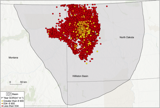
Fig. 7. Production data for the Bakken and Three Forks formations of the Williston Basin [82]. |
The Bakken Formation consists of upper and lower organic-rich black shales separated by a middle member of calcareous siltstone [93-94]. Hydrocarbons are generated in the Upper and Lower Bakken shales, but produced from the either the Middle Bakken or the upper part of the underlying Three Forks Formation [93]. The Middle Bakken consists of a mixed sequence of carbonates and siliciclastics [94]. In the Elm Coulee field in Montana, the Middle Bakken reservoir is a fractured dolomite reservoir [13,15], but, in general, laminated sandstone/siltstone facies are the best reservoir facies in Middle Bakken [93]. The upper Three Forks consists of silty to sandy dolomite, dolomitic siltstones, and gray-green shales [93,95]. The Middle Bakken is the thickest of the producing intervals, reaching a maximum of about 24 m, while the upper Three Forks is at most 15 m thick [93].
2.1.4. Late Mississippian shale plays
2.1.4.1. Barnett shale
The Late Mississippian of the southern Laurentian margin has several shale plays, including the Barnett shale. As discussed previously, the Barnett shale of the Fort Worth Basin was the first shale gas play to be extensively developed in the United States. Production in the core Barnett play is dominated by dry gas, with increasing oil to the north and west (Fig. 8 ). The Fort Worth Basin Barnett play covers about 27 000 km2 and has produced from more than 15 800 wells. The Barnett shale is also prospective, but less developed, in the Permian Basin, with an area of 17 600 km2 and 128 wells that have reported production (Fig. 8 ). The western part of the Delaware Basin appears dominated by gas and gas-condensate, while the western part of the Midland Basin appears more oil prone.
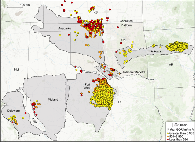
Fig. 8. Production data for Barnett shale (Forth Worth, Midland and Delaware), Mississippi (Meramec/Sycamore) Lime (Anadarko & Cherokee Platform), Caney shale (western Arkoma, Ardmore, and Marietta) and Fayetteville shale (eastern Arkoma) [82]. CBP—Central Basin Platform, KS—Kansas, OK—Oklahoma, AR—Arkansas, TX—Texas, NM—New Mexico. |
The Barnett shale of the Fort Worth Basin consists of laminated siliceous mudstone, laminated argillaceous lime mudstone (or marl), and argillaceous lime packstone [70]. The lower part of the Barnett is locally gradational into the shallow water Chappell Limestone [70]. To the northeast, the Barnett reaches thicknesses greater than 300 m and contains a series of carbonate debrites [43], with an average of 85 m [65]. In northeasternmost part of the basin, the Barnett can be subdivided into upper and lower members separated by the Forestburg limestone, a carbonate interval up to 60 m thick, but over much of the basin, the Barnett is not internally differentiated [43]. The Barnett was deposited on an angular unconformity, which impacts the prospectivity of the play, as to the south and west, the Barnett shale directly overlies karsted Ellenburger carbonates that may be water-bearing [43], creating a potential issue during fracture stimulation.
The Barnett shale in the Permian Basin overlies an Early Mississippian (Kinderhookian to Osagian) limestone that, in the Delaware Basin, thickens to the north and east [96-97]. The Late Mississippian (Meramecian to Chesterian) Barnett itself transitions from basin shales to shelf carbonates moving north into New Mexico [97]. In the subsurface of the northern Delaware Basin, the Barnett can be subdivided into a lower carbonaceous shale and an upper siliciclastic shale based on a pronounced change in gamma-ray signature, while the lower unit can be further subdivided by resistivity characteristics [96]. Based on limited core data, the Barnett in the Delaware Basin consists of laminated mudrock, micro-laminated mudrock, unlaminated mudrock, and argillaceous mudrock [98]. The thickness of the lower Barnett increases from above 60 m to more than 200 m, moving from west to east across the Delaware Basin, while the upper Barnett reaches a thickness of ~about 65 m in the central Delaware Basin [96].
2.1.4.2. Fayetteville shale and Caney shale
The Fayetteville shale lies within the eastern Arkoma Basin of Arkansas and is approximately equivalent in age to the Barnett shale [7,99]. In 2002, geologists of Southwestern Energy calculated that a conventional sandstone reservoir within the Arkoma Basin was producing more gas than could be explained and surmised that the underlying Fayetteville Shale may have been contributing to production [99]. After determining that Fayetteville shale properties were similar to those of the Barnett Shale, Southwestern drilled and completed the Fayetteville discovery well in 2004 [99]. Fayetteville production is entirely dry gas (Fig. 8 ). The play covers 6 000 km2 [65] and has reported production from about 7 300 wells.
The Fayetteville consists of black, fissile, and locally calcareous mudrock with interbedded calcareous mudstone [34]. Fayetteville thickness is 18 m to 215 m, with an average thickness of 90 m [65]. Towards the northern edge of the Arkoma Basin, the shale grades upward and northward into limestone. Away from the basin edge, the shale grades upward into lime mudstone (to the east) or siltstone (to the west) [34]. The lower part of the Fayetteville is the main target interval [34,99] and is distinguished from the upper Fayetteville by higher radioactivity (based on gamma-ray response) [67].
The Caney shale in Oklahoma is the age equivalent of both the Fayetteville and Barnett shales. Although the Caney shale has been drilled in both the Arkoma and Ardmore basins, it has not seen the same level of development [100]. Caney shale wells, particularly those in the Arkoma Basin, showed poor production rates, largely due to high clay content limiting the impact of hydraulic fracturing [100-101]. Drilling in the Ardmore Basin of southern Oklahoma, has shown more promise, but the best producing wells are those completed in interbedded limestone and siltstone facies within the shale [100]. Production from the Caney in the Arkoma Basin is dry gas, while there is both oil and gas production from the Caney in the Ardmore and Marietta basins (Fig. 8 ). S&P Global reports production from 109 Caney Shale wells: 59 in the Ardmore Basin, 29 in the Arkoma Basin, 18 on the Cherokee Platform, and 2 in the Anadarko Basin [82].
2.1.4.3. Late Mississippian carbonates
Late Mississippian (Meramecian) carbonates in Oklahoma are the shelfal equivalents of the Barnett/Caney shales and have produced as conventional reservoirs since 1904 in areas along the Oklahoma-Kansas border [102]. By the 1960s, industry focus had moved to fracturing vertical wells to develop tighter Mississippi (Meramec) lime reservoirs of the Sooner Trend in the northeastern Anadarko Basin [102-103]. Around 2010, there was a notable increase in activity with unconventional drilling technologies applied to develop lower permeability reservoirs in the play areas known as the STACK (Sooner Trend Anadarko (Basin) Canadian Kingfisher counties) and the SCOOP (South Central Oklahoma Oil Province) of the Ardmore Basin [102⇓-104]. Meramec reservoirs in the STACK consist of silty limestones, calcareous to argillaceous siltstones, and organic-rich mudstones that were deposited on a lower shoreface ramp [104]. The Meramecian section in the SCOOP area consists of the Caney shale and the underlying Sycamore limestone which were deposited in a deeper-water setting than the Meramec of the northern Anadarko Basin [104]. The Sycamore consists of calcareous siltstone, cherty mudstone, and thinly-bedded shale, with the siltstones representing turbidite flows into deeper water setting [104]. Production from both areas is oil-rich (Fig. 8 ), and about 1 300 productive wells have been drilled in these intervals since 2001. Given that this interval is also present in the Permian Basin [96-97], it may be prospective there as well, but there does not appear to be any recorded production to date.
2.1.5. Permian shale plays
Shale plays of Permian age are restricted to the Permian Basin area of west Texas and southeastern New Mexico. The Permian Basin is unusual in the number of unconventional reservoir targets that exist in the area. Most shale plays have one or two potential reservoir intervals, but 11 separate intervals have seen at least some production in the Permian Basin, not including the deeper Woodford and Barnett intervals already discussed. Shale oil and gas production in the Permian Basin largely comes from the Latest Pennsylvanian to Early Permian basinal facies within the Delaware and Midland basins, primarily the Wolfcamp “Formation” and the Leonardian Spraberry (Midland Basin) and Bone Springs (Delaware Basin) units (Fig. 9 ), sometimes known as the Wolfberry [105] and Wolfbone [106] plays. Current industry definition of the Wolfcamp “Formation” covers an interval from the latest Pennsylvanian to the earliest Leonardian (Cisco shale or Wolfcamp D through Lower Leonard or Wolfcamp A). The Wolfcamp interval is composed of a mix of carbonaceous mudrocks with local carbonate intervals and siliceous mudrocks [105]. The remainder of the Leonardian interval (Wolfcamp A and above) is composed of alternating lowstand sequences dominated by siliciclastics, especially laminated siltstones and highstand sequences dominated by calcareous mudrocks [105]. Intervals dominated by calcareous mudrocks are the most organic-rich, but thin mudrocks interbedded with siliciclastics may also have significant organic content.
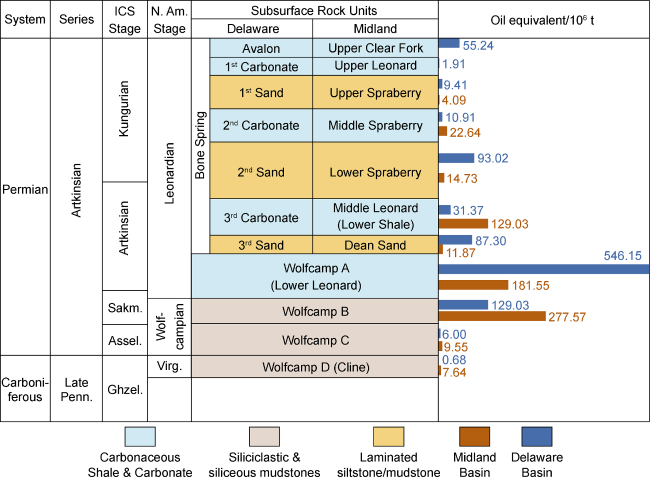
Fig. 9. Stratigraphic comparison of the Wolfcampian and Leonardian sections in the Midland and Delaware basins, and volumes produced from each interval [109]. |
The Wolfcamp section alone is significantly thicker than most shale plays, which generally have an average thickness of less than 100 m [65]. Based on recent interpretation [107-108], the Wolfcamp of the Midland Basin averages 648 m thick, with a maximum thickness of 1 850 m, while the Wolfcamp of the Delaware Basin with greater accommodation space during deposition, has an average thickness of 786 m and a maximum thickness of about 2 900 m. The Wolfcamp is informally divided into four units (Fig. 9 ), among which each unit may have stacked production. The Leonardian section (not including the Wolfcamp A) averages 245 m thick in the Midland Basin, and 725 m thick in the Delaware Bain.
The Wolfcamp A and B are the main producing intervals in both basins (Fig. 9 ). Above the Wolfcamp A, there is a difference between the two basins in producing intervals. In the Delaware Basin, it is the siliciclastic-rich “sand” (lowstand) units within the Bone Springs Formation that have the highest production, but in the Midland Basin, the mudstone and carbonate-rich lowstand intervals of the Middle Leonard and Middle Spraberry that have the highest production.
Production in the Midland Basin is dominantly oil, with Leonardian production being more areally restricted than Wolfcamp production (Fig. 10 ), as the thick portions of these intervals became increasingly confined to the basin depo-center as the basin was filled during the Leonardian. Production in the Delaware Basin is a mix of oil and gas, with gas increasing to the west. S&P Global reports production from more than 18 900 horizontal wells in Wolfcamp and Leonard reservoirs. Most wells (12 822) produce from the Wolfcamp and about 60% (11 425) are in the Delaware Basin [82].
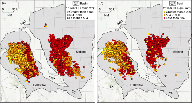
Fig. 10. Production data for Wolfcamp “Formation” (Delaware Basin) (a) and Bone Springs + Spraberry/Dean formations (Midland Basin) (b) [82]. CBP—Central Basin Platform, SC—Sheffield Channel, SSC—San Simon Channel, NM—New Mexico, TX—Texas. |
2.2. Mesozoic plays
2.2.1. Haynesville shale
In 2004, KCS Resources drilled a vertical well which had significant gas shows in the Haynesville/Bossier shale interval [110]. Over the next several years, several operators drilled vertical wells to collect and analyze core samples in the play [110-111]. The first horizontal well was completed by Chesapeake in 2007 with an initial production rate of 7.28×10⁴ m3/d [111].
The Haynesville shale is an organic-rich, carbonaceous mudstone that was deposited in a semi-restricted portion of the Gulf Coast Basin during the late Jurassic [50]. The section was originally named the Lower Bossier Formation, but was called the Haynesville shale by Chesapeake Energy because it is correlative to the Haynesville limestones that were deposited on carbonate platforms surrounding the shale basin [50]. However, there is also production from the overlying Bossier shales and the names have sometimes been used interchangeably [112].
There are two Haynesville shale depocenters separated by a carbonate platform: one in the East Texas Salt Basin, and one along the Texas-Louisiana Border, covering part of the Sabine uplift and into the North Louisiana Salt Basin [50]. Haynesville shale thickness is at its highest in the northern part of eastern depocenter where it reaches 120-130 m [50]. Average thickness in that depocenter is 60 m [65]. In the East Texas Salt Basin, the Haynesville shale is generally thinner (less than 30 m), but does reach 60 m in the southwestern portion of the depocenter [50]. Haynesville shale composition varies across the basin, with the mudrocks being more calcareous to the south and west, and having greater siliciclastic input to the north and east [50]. Influence of siliciclastic sediments also increases upward, with the overlying Bossier shale being dominated by sediments fed into the basin by prograding delta [113]. There are three main facies within the Haynesville shale: unlaminated peloidal siliceous mudstone, laminated peloidal or siliceous mudstone (most common), and bioturbated calcareous or siliceous mudstone [50]. For the overlying Bossier shale, facies consist of massive argillaceous mudrocks, bioturbated argillaceous mudrocks and argillaceous claystones, all of which have significantly lower carbonate content than similar Haynesville facies, and also have generally lower organic matter content [113].
Historically, the Haynesville shale play has been restricted to the eastern (Sabine Uplift) depocenter, but in the last few years, a new play area (the western Haynesville Play) has opened up in the southwestern part of the East Texas Salt Basin. Over 6 000 producing wells have now been drilled in the core Haynesville Play (Fig. 11 ), while the new play area (the western Haynesville) currently has production reported from 11 wells. Haynesville production is dominantly dry gas, but some oils have been produced toward the northern edge of the core area.
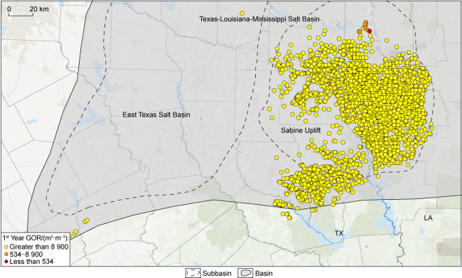
Fig. 11. Production data for Haynesville-Bossier shales [82]. TX—Texas, LA—Louisiana. |
2.2.2. Eagle Ford Group
It has been reported that Petrohawk Energy discovered the Eagle Ford Group shale play in 2008 [114-115], but the history is more complex. Between 1960 and 2003, 12 wells reported production from the Eagle Ford Group, but these wells were all targeting deeper formations, and completed in the Eagle Ford after encountering gas. Most were vertical wells and the cumulative production of all twelve is 2.65×10⁴ t of oil and 5.9×10⁶ m3 of gas [82]. Most of these wells were in Maverick County, towards the northwestern edge of the modern (U.S.) Eagle Ford play, but there were also two wells in Webb County, and two in Gonzales County [82] (Fig. 12 ). Between 2005 and 2008, Burlington Resources (later ConocoPhillips) and Texas Crude tested the Eagle Ford in the Karnes Trough area while TXCO Resources, Espada Operating, and Cornerstone Exploration and Production drilled wells in Eagle Ford in the Maverick sub-basin [82] (Fig. 12 ). In total, from 2005 until the spudding of Petrohawk’s STS-1 Hawkville discovery, there had been 15 wells drilled in the Eagle Ford play.
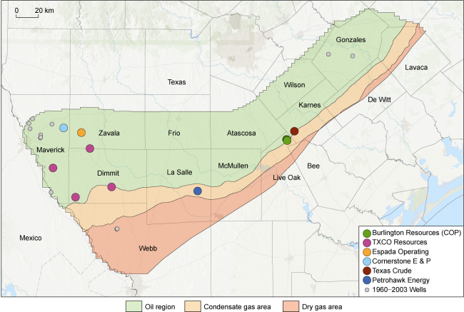
Eagle Ford production is a mix of oil, gas with condensate, and dry gas that stretches from slightly east of the San Marcos Arch, to the Mexican border (Fig. 13 ). The southern margin of the play parallels the Early Cretaceous Sligo reef margin, across which the Eagle Ford deepens and thins, while the northern margin of the play is the northern limit of the Eagle Ford oil window [51]. Northeast of the San Marcos Arch, significant facies changes occur due to increasing siliciclastic input from the Woodbine Delta, limiting the extent of the play [51,53]. Over 25 700 wells have reported production from the Eagle Ford [82] since 2005.
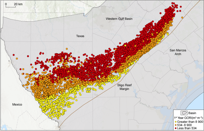
Fig. 13. Production data for the Eagle Ford shale [82]. |
A Cenomanian-Turonian (Late Cretaceous) marine transgression led to deposition of the organic-rich carbonaceous mudstones and limestones of the Eagle Ford Group [51]. The lower Eagle Ford is a transgressive sequence, capped by a condensed section, while the upper Eagle Ford represents a highstand sequence [51]. While the Eagle Ford is described as a shale formation, in outcrops to the north and west of the play, it is a mix of organic- rich coccolithic argillaceous wackestone and organic-poor pelagic grainstone [116-117]. The Eagle Ford averages 27 m thick and reaches a maximum thickness of 78 m and the play covers an area of almost 36 000 km2 [65].
2.2.3. Niobrara Formation
The Niobrara Formation was deposited during the same marine transgression as the Eagle Ford Shale (Late Cretaceous: Cenomanian-Turonian) over a large area (more than 130×104 km2) of the Western Interior Cretaceous Seaway [59,118]. The Niobrara is dominantly composed of interbedded chalks and organic-rich calcareous mudrocks [118-119], although clastic content increases from east to west [64]. To the east, the Niobrara sits unconformably on non-calcareous shales (Carlisle, Benton), although locally there is an intervening sandstone between the underlying shale and the Niobrara [25,118]. The Niobrara is overlain by another interval of non-calcareous shale (Pierre shale to the east) [25,64,119]. To the west, both the overlying and underlying shales are assigned to the Mancos shale and the Niobrara intertongues with and grades into the Mancos [25,119]. Both the Mancos and Pierre shales have been considered as potential shale plays [16], but neither has been developed.
Production from fractured a Pierre shale reservoir (sourced by the Niobrara) began in 1881 at the Florence-Cañon City Field and the first Niobrara production began in 1924 at the Tow Creek Field [64]. In 1970, the giant Wattenberg Field in Colorado was discovered by Amoco with production initially from an Early Cretaceous sandstone, and beginning from the Niobrara in 1985 [120]. The Niobrara was known to be a tight reservoir with existence of natural fractures necessary for production [59]. During the 1990s, there was an initial spurt of horizontal drilling [82] (Fig. 14 ), likely attempting to intersect a greater number of natural fractures. Renewed interest in horizontal drilling (with hydraulic fracturing) began in 2008, peaking in 2014 and 2019 [82] (Fig. 14 ).
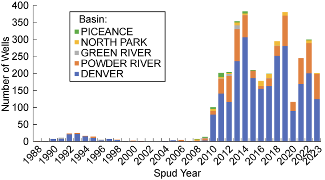
Fig. 14. Stacked bar chart of horizontal wells targeting the Niobrara Formation in 1988-2023 [82]. |
Although the Niobrara Formation and the basins it produces from cover parts of 8 states, reported production from horizontal wells in Niobrara is restricted to Wyoming and Colorado (Fig. 15 ). Production is concentrated in the Denver Basin (2 600 wells), followed by the Powder River Basin (747 wells) and North Park Basin (89 wells) [82]. Production in these basins is dominated by oil with lesser gas. The Green River and Piceance basins each have production from about 30 wells and are generally gassier, with the Piceance producing mainly dry gas.
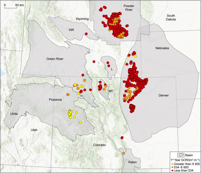
Fig. 15. Shale oil and gas production data for the Niobrara Formation. L—Laramie Basin, NP—North Park Basin, WR—Wind River Basin. |
3. Resources and production
Basin-scale resource assessment has long been used to identify focus areas and evaluate acreage. The continuous nature of unconventional plays makes them well suited for this type of assessment, as one does not need to consider long distance migration or trapping. A common methodology is to define assessment areas within the play and run Monte Carlo simulations for thickness, porosity, water saturation and other parameters [1-2,121]. This methodology provides a range of potential resource, particularly in areas where there is little data available, and it can be done relatively quickly. The disadvantage is that it does not differentiate between different areas within the play other than the pre-defined assessment areas. This methodology cannot highlight areas that have better rock properties or better resource concentration.
A more deterministic approach to resource assessment is applied by the Tight Oil Resource Assessment (TORA) research consortium at the Bureau of Economic Geology, part of the Jackson School of Geosciences at the University of Texas at Austin. This foundation of this approach is geologic reservoir characterization [65,122], including structural, stratigraphic and facies analysis [65,109,122], petrophysical analysis [62,108,122], 3D geological modeling [107-108] and estimation of in-place resources [122-123]. Once in-place resources are assessed, the results are combined with production analysis (decline, estimated ultimate recovery, spacing and interference), and productivity analysis (production drivers) to generate estimates of technically recoverable resources (TRR) and how they vary across the play [124-125]. These, in turn, feed into economics analysis and development of production outlooks [122,126].
TORA has evaluated and estimated technically recoverable resources for eight shale plays across the United States: Eagle Ford Shale, Haynesville Shale, Midland Basin, Delaware Basin, Barnett Shale, Fayetteville Shale, Bakken/Three Forks and Marcellus Shale (Fig. 16 , Table 2 ). Values for the Delaware Basin are only reported for the Wolfcamp A, Wolfcamp B, and 3rd Bone Springs Sand, while Midland Basin values are only for the Wolfcamp A and B. These models have been recently updated and once analysis has been completed, both in-place and recoverable resources should increase. Both the U.S. Geological Survey (USGS) and a consortium at West Virginia University (WVU) conducted resource assessments on the Utica shale using the same probabilistic method, but with different inputs [121,127]. TRR estimates for gas from WVU study are significantly higher than those from the USGS assessment (Table 2 ), which likely stems from differences in the estimated productive areas between the two assessments: WVU used smaller ranges, but higher means for their productive area inputs when compared to the USGS assessment.
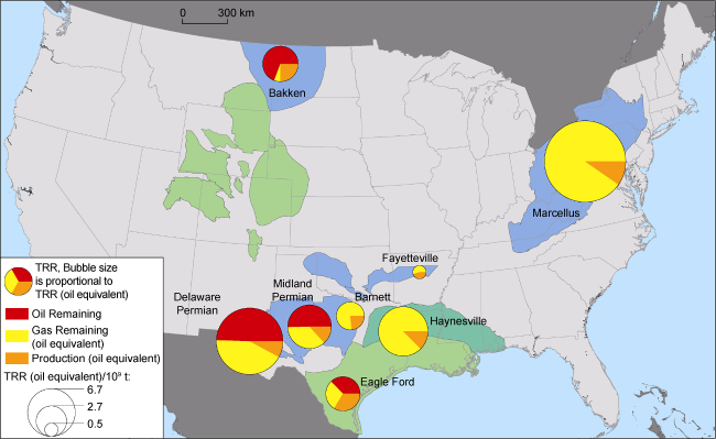
Fig. 16. Estimates of technically recoverable resource (TRR) for shale plays analyzed by the TORA consortium at the Bureau of Economic Geology [82]. |
Table 2. Resource assessment results and produced volumes for some major U.S. shale plays |
| Shale play | In-Place volumes | TRR | Produced volumes | |||
|---|---|---|---|---|---|---|
| Oil/ 109 t | Gas/ 1012 m3 | Oil/ 109 t | Gas/ 1012 m3 | Oil/ 109 t | Gas/ 1012 m3 | |
| Eagle Ford shale | 40.9 | 12.7 | 1.91 | 1.85 | 0.64 | 0.63 |
| Haynesville shale | 19.6 | 8.76 | 1.09 | |||
| Midland | 94.0 | 15.6 | 3.27 | 2.80 | 0.48 | 0.31 |
| Delaware | 73.1 | 32.2 | 6.96 | 7.28 | 0.58 | 0.54 |
| Barnett | 14.2 | 2.80 | 0.01 | 0.65 | ||
| Fayetteville | 2.1 | 0.64 | 0.29 | |||
| Bakken | 26.9 | 43.4 | 3.24 | 0.52 | 0.71 | 0.27 |
| Marcellus | 61.6 | 23.70 | 0.02 | 2.26 | ||
| Utica (WVU) | 11.3 | 89.4 | 0.27 | 21.69 | 0.03 | 0.56 |
| Utica (USGS) | 0.38 | 3.28 | ||||
Note: All but the Utica Shale assessments were done by the TORA consortium at the Bureau of Economic Geology, UT-Austin. |
As shown earlier in Fig. 1 , production from shale plays made up 62% of total U.S. oil and gas production by the end of 2023. Since 2007, combined shale oil and gas production has risen from about 11.2×10⁴ t/d of oil equivalent to more than 300.0×10⁴ t/d (Fig. 17 ). Over the same time period, non-shale oil equivalent production dropped from about 217×104 t/d to a low of 152×104 t/d in September 2021. Shale production in U.S. first exceeded conventional production in August of 2017 and has remained higher since that time. Interestingly, at that time, non-shale production also began to show a slight increase.
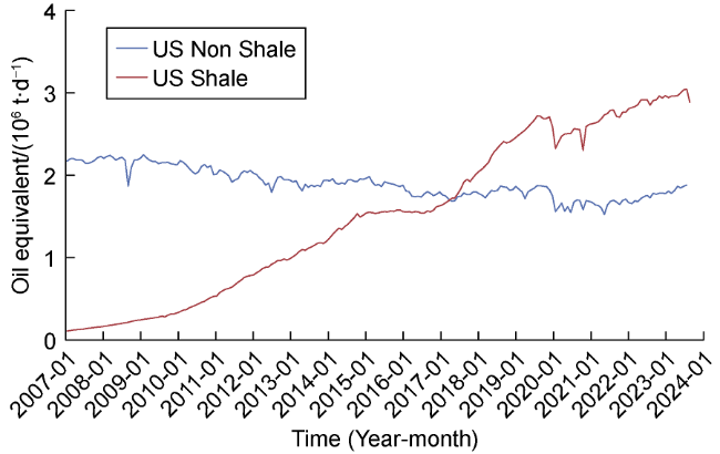
Fig. 17. Combined U.S. oil and gas production over time comparing production from shale plays to non-shale production [16]. |
After a sharp drop in both shale and non-shale production in early 2020, due to the COVID-19 pandemic, both shale and non-shale production have started increasing again, although non-shale production took longer to recover from that reduction. The recent increase in non-shale production is the reason that shale production has remained at ~60% of total for the last several years.
Looking only at oil, shale production rates increased slowly until mid-2010, when a rapid increase began that continued through the first quarter of 2015, largely driven by production from the Eagle Ford shale, although oil production rates in both the Bakken and Permian were increasing over the same time period (Fig. 18 ). Beginning in late 2014, oil prices began to plummet, with the West Texas Intermediate benchmark price dropping from about \$106/bbl to \$47/bbl in six months, ultimately reaching a low of about \$30/bbl in early 2016. This price drop led to reduced production rates through September 2016, largely driven by the Eagle Ford. In the Permian Basin and Anadarko Basin, production did not decrease, but the rate of increase slowed. By early 2017, oil production rates were increasing again, with the largest increase coming from the Permian Basin. Production rates from both the Anadarko Basin and the Niobrara Formation began to fall in the second half of 2019, with a sharp across the board reduction in early 2020. Since then, production rates have continued to increase in the Permian Basin, but have stayed relatively flat in the other shale oil plays, although rates in the Bakken and Niobrara did show an upward trend in the second half of 2023. Oil production is dominated by the Permian Basin at about 68.5×10⁴ t/d of oil, accounting for 63% of shale oil production (about 108×104 t/d) and 38% of total U.S. production (about 182.0×10⁴ t/d).
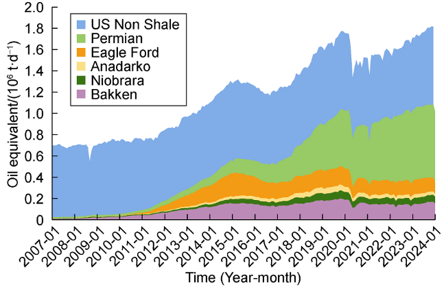
Fig. 18. U.S. oil production rates from shale oil plays and non-shale plays [16]. |
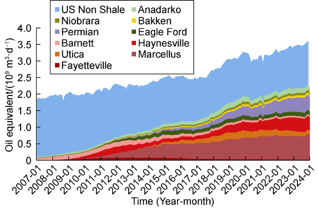
Changes on shale gas production rates over time are similar to those of shale oil, although gas rates began increasing slightly earlier than shale oil rates, with Haynesville production coming on in 2009, followed by the Marcellus shale in 2011 (Fig. 19 ). Shale gas production rates are complicated by the significant volumes of gas produced from shale oil, with shale oil plays currently contributing about 38% of shale gas production. Since the gas produced from these plays is tied to oil price, rather than gas price, the economic drivers are different, which may cause issues for the gas producers. One can see the effect in Haynesville shale gas production (Fig. 19 ) where production decreases starting in 2012. The increasing amount of gas on the market from shale oil plays was driving the domestic gas price down, leading to reduction in Haynesville development activity. After liquefied natural gas (LNG) shipments from the Gulf Coast began in 2016, development activities of Haynesville shale began to increase and leading to increasing Haynesville production rates. At the end of 2023, the Marcellus was the dominant shale gas producer (about 7.76×10⁸ m3/d), followed by the Permian Basin (about 4.64×10⁸ m3/d), and the Haynesville (about 4.26×10⁸ m3/d). Together these accounted for 73% of U.S. shale gas production (about 2.8×10⁸ m3/d) and 47% of total U.S. gas production (about 36.1×10⁸ m3/d). Recently, operators have begun to curtail production in the Haynesville and Marcellus, looking to reduce the gas surplus on the market, as gas prices have dropped following a warm winter [128].
Fig. 19. U.S. gas production rates from shale plays and non-shale plays [16]. |
4. Recent/emerging trends
Development of shale oil and gas has been largely driven by advances in technology, particularly in the drilling and completion space [8,10 -11,15]. One of the more recent focuses has been a push towards “cube development” or “co-development”. The idea behind cube development is to develop multiple stacked benches within a full section (1 square mile area) by drilling and completing the entire subsurface “cube” at the same time [129-130]. The goal is to reduce parent-child development issues, where in-fill wells (child wells) have poorer production performance compared to the initial wells in the area (parent wells) due to reservoir depletion from production of the original wells. Cube development has a large up-front cost, which tends to limit its use to larger companies [130]. There are also some issues with these developments, as choosing a well spacing that is too small may reduce the single-well production, counteracting the potential cost benefit from taking this approach [131-132]. Nevertheless, ExxonMobil claims that this method gives them 30%-50% greater net present value than the approach of drilling the best bench first [130].
Operators are also looking at ways to increase production from older wells. One approach is to refracture older wells to re-stimulate production. Completion designs in early shale wells were significantly different from modern completions, possibly using wide cluster spacings or high viscosity fluids, resulting in lower single-well recovery than modern wells [133⇓-135]. Refractured wells allow recovery of bypassed resources without the cost of drilling and completing another well in the same area [133].
Enhanced oil recovery (EOR) is another approach that is gaining attention as a method to increase production from unconventional reservoirs, although pilot projects have not always been successful. EOG Resources conducted its first EOR test in the Eagle Ford in 2012, with their first significant project beginning in 2014 [136]. By 2021, there were 34 Eagle Ford EOR projects that had been permitted by 8 operators, with EOG Resources operating more than half of these [137]. These projects largely use the technology of cyclic injection of natural gas (sometimes called huff-and-puff) where a miscible gas is injected into the horizontal well (huff), the well is then shut in for a period of time to allow the injected gas to mix with the oil (soak), and then the well is put back on production (puff) [138]. Results are difficult to determine, as the operators have not published them, and Texas production report is done by lease rather than by well. One attempt to use publicly available data and simulations to estimate performance suggested 30%-50% improvement on oil recovery over 10 years [136]. There have been limited tests on injection of carbon dioxide rather than natural gas for huff-and-puff EOR operations. Results from tests in the Bakken have shown mixed to poor results [139], while results from a test in the Eagle Ford showed more promise [140].
One of the more recent trends, is the drilling of horseshoe or U-shaped wells, where there are, after the vertical section, two lateral sections connected by a U-turn section. Previously, wells described as U-shaped have been drilled for coal bed methane in China [141-142] and offshore heavy oil in the Congo [143], but these wells are U-shaped in cross-section and straight in map view. The first U-shaped well was drilled by Shell in 2019, but was not planned that way [144]. During drilling of the vertical section of a well in the Delaware Basin, there were excessive mud losses and the vertical section had to be abandoned, so the engineering team extended another horizontal well, turning 180°, and drilling a new lateral section along the abandoned well trajectory [144]. Both horizontal sections were completed, but the U-turn was not, and the operation saved on both rig time and total cost compared to drilling two wells [144]. In 2020, Chesapeake drilled a U-turn well in the Eagle Ford shale, aiming to maximize lateral length in a tight lease space [145]. In 2023, Matador Resources conducted a pilot project in the Delaware Basin, drilling two horseshoe wells rather than four horizontal wells in one section, saving about $1×10⁷ and seeing production performance on par with that expected from four horizontal wells [142]. Evaluation of well paths from S&P Global’s data base [82] indicates that, in addition to the Shell and Matador wells, another five horseshoe wells have been drilled in the Delaware Basin. Since the completion of Chesapeake well in 2020, six additional horseshoe wells have been drilled in the Eagle Ford. The last year has also seen one horseshoe well drilled in the Midland Basin and another in the Marcellus Shale.
5. Conclusions
While production from naturally-fractured shales has long contributed small volumes to U.S. hydrocarbon production, over the last twenty years, production from shale reservoirs has become the dominant source of total U.S. hydrocarbon production. This was not an instantaneous process; there had been more than twenty years of concerted efforts to develop shale resources prior to development of technology that allowed for hydraulic fracturing of horizontal wells kicked off the “shale boom” in the United States.
Major shale reservoirs in the U.S. range in age from Silurian to Late Cretaceous, including Middle Ordovician, Middle to Late Devonian, Early Carboniferous (Middle to Late Mississippian), Early Permian, Late Jurassic and Late Cretaceous (Cenomanian-Turonian). Depositional settings include intra-cratonic basins, foreland basins and passive margins.
While some shale reservoirs were deposited at approximately the same time period and in similar depositional settings, the regional extent of these plays leads to differences in facies and mineral components that result in changes in productivity potential across the play. Looking in detail at individual plays shows that “shale reservoirs” are often not only shale, shale oil may be produced from carbonaceous mudrocks or interbedded cherts, carbonates, or siltstones interbedded in a sequence of organic-rich mudstones.
Shale resources in the United States are significant, with in-place estimates of over 0.246×10¹² t of oil and over 290×1012 m3 of natural gas and recoverable estimates of over 150×108 t of oil and over 50×1012 m3 of natural gas. It is worth pointing out that recoverable resource is a dynamic target that tends to increase as technology develops.
Production from U.S. shale plays has been on a generally upward trend since around 2010 and surpassed conventional U.S. production in 2017. Reduction in demand or increased supply globally has led to reductions in commodity prices, which reduces the production. Shale production is more sensitive to continued capital investment. Reducing the number of wells completed each year has a stronger effect on shale plays than on conventional plays. Production from dry-gas shale plays is particularly sensitive to demand and availability of offtake solutions, such as LNG, as shale oil plays produce significant amounts of gas as well.
Operators continue to search for new approaches to maximize returns on their acreage. Over the last several years, there has been increased focus on developing the entire stack of producing benches (cube development) and methods to increase production rates from pre-existing wells (EOR, refracturing). While there has long been a focus on increasing lateral length to boost productivity, operators are now looking at achieving that though drilling multiple lateral sections on a single well (horseshoe or U-shaped wells).
From the geological or engineering point of view, given the large resource base and continuous technological development, shale oil and gas production will continue to increase for many years. We see this in the testing of the Woodford and Barnett plays in the Permian Basin, and the extension of the Haynesville play into the East Texas Salt Basin, as well as continued efforts to develop effective EOR strategies. Challenges to continued production are generally economic, particularly when commodity prices are low, as maintaining shale production requires continued capital investment.
Acknowledgements
This work was supported by the State of Texas Advanced Resource Recovery (STARR) program, and the Bureau of Economic Geology’s Tight Oil Resource Assessment (TORA) and Mudrock Systems Research Laboratory (MSRL) consortia. Access to well and production data was provided by S&P Global.