

Introduction
Accurate reservoir performance prediction is vital for residual oil extraction and enhanced crude oil recovery[1⇓⇓-4]. Commonly used prediction techniques include geological methods, reservoir engineering methods, and numerical simulations [5]. However, due to the high cost of direct measurement and the nonlinearity and multi- variables of control equation, the solving efficiency of discrete equations is generally lower [6-7]. In the process of history matching and subsequent production optimization, thousands of numerical simulations are needed for reservoir performance prediction, which consumes considerable time [8-9]. It is in urgent need to establish a new efficient reservoir performance prediction method to effectively address the limitations of traditional prediction methods like high test expense, ideal assumption and great calculation cost.
Currently, data mining and artificial intelligence are increasingly applied in various industrial fields and have achieved remarkable results, presenting opportunities for the digital transformation of the traditional petroleum industry [10⇓-12]. Their application in petroleum field at present stage includes geological model parameterization [13-14], geoscientific modeling [15-16], fluid property prediction [17], well production prediction [18-19], sweet-spot detection [20], and shale gas recovery calculation [21-22]. Deep learning [23], renowned for its efficacy in modeling nonlinear relationships and its capabilities in automated learning and abstract feature extraction from input data, facilitates more complex mapping and characterization. This offers innovative approaches for constructing surrogate models aimed at predicting reservoir performance for automatic history matching [24-25] and production optimization [26⇓⇓⇓-30]. Zhu et al. [31] constructed a Bayesian deep Convolutional Neural Network (CNN) to quantify geological uncertainty. Tripathy et al. [32] developed a single-phase flow forward simulation surrogate model, while Laloy et al. [33] built the same model using Generative Adversarial Networks (GAN), in which the high-dimensional projections are determined by training two adversarial neural networks. Wang et al. [34] proposed a neural network for predicting single-phase flow in two-dimensional porous media under theoretical guidance. Zhong et al. [35-36] used GAN to construct a surrogate model to simulate reservoir pressure and fluid saturation. Ma et al. [37-38] combined a CNN and Long Short-Term Memory (LSTM) to predict the production data, which reduced the additional computation caused by images. Jin et al. [39] proposed the embedded control (E2C) framework to predict well response and dynamic evolution of 2D heterogeneous reservoirs in different well control conditions without considering geological uncertainty. Wei et al. [40] used the ConvLSTM model to predict oil saturation and bottom-hole pressure distribution at different production moments using actual oilfield data. Zhang et al. [41] employed vector-type features and high-dimensional spatial-type parameters as CNN input to predict pressure and oil saturation. Huang et al. [42] constructed a deep-learning surrogate model for the rapid 3D simulation of actual reservoirs. Although this model takes into account different well control conditions, it does not fully consider the uncertainty of production time.
Deep learning can better describe complex mapping and effectively characterize the spatial and temporal features of reservoir performance simulation, compared with traditional reservoir performance prediction techniques. Practical development requires the periodic adjustment of the production program for long-term water injection alters the physical properties of reservoirs. The existing deep learning surrogate models generally predict reservoir performance at certain moments under fixed well control conditions based on static geological models, without fully considering the geological conditions and well-control uncertainties during the evolution of reservoir performances, so they cannot predict reservoir performance in time-varying, well-control, and uncertain geological settings. To this end, this paper proposed to delineate the issue of reservoir performance prediction within manifold space and to develop an intelligent surrogate model for reservoir performance prediction utilizing the Conditional Evolutionary Generative Adversarial Network (CE-GAN). This model comprehensively accounts for the temporal and spatial change characteristics of reservoir performance under the condition of geological uncertainty and time-varying well control conditions. Therefore, it can rapidly forecast reservoir performance in time-varying well-control scenarios.
1. Definition of the surrogate model for reservoir performance prediction
Numerical simulation is typically used in traditional reservoir development to solve the problem of oil-water two-phase seepage in porous media, simulate subsurface oil and water flow, and obtain fluid and pressure distribution characteristics at different production moments, thus predicting reservoir production performance. This study developed a surrogate model based on deep learning, which can predict reservoir performance without complex history matching. According to the literature [43], the surrogate model for reservoir performance prediction is expressed via a forward model as shown in Eq. (1):
This model aims to replace the traditional numerical simulator in a cost-effective, non-invasive manner. The reservoir performance prediction is transformed into a regression problem concerning the reservoir performances map influenced by time-varying well control, by researching reservoir performance prediction from the perspective of generative modeling. Note that the “map” mentioned was matrix composed of actual reservoir performance values. For example, a saturation map represented a matrix of saturation distribution data in which each element had a physical meaning. The surrogate model can effectively predict reservoir performance by learning the nonlinear relationship between the initial state of the reservoir and states at any subsequent moment. The surrogate model for reservoir performance prediction is defined as the regression model shown in Eq. (2). Here, nb represents the number of grids in the reservoir model, and denotes the set of pressure and oil saturation at moment t.
${{x}_{t+1}}=\hat{f}\left( {{x}_{t}},\Lambda,{{c}_{t}},\xi ;\gamma \right)$
2. Construction of the surrogate model for reservoir performance prediction
2.1. Reservoir performance prediction surrogate model based on CE-GAN
This paper constructed a surrogate model for reservoir performance prediction based on CE-GAN (Fig. 1 ), and defined that the reservoir performances map under time-varying well-control is located in a high-dimensional manifold space. In the surrogate model, the spatial changes of the reservoir performances map are characterized on the basis of the reservoir physical properties and well control parameters, and accordingly the evolution laws of the reservoir performance map over production time were studied. Thus, the issue of reservoir performance prediction is transformed into an image evolution problem based on permeability distribution, initial reservoir performances, and time-varying well control, which improves prediction speed and accuracy.
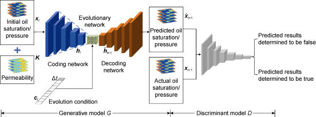
Fig. 1. The structure of the CE-GAN surrogate model. |
Based on the conditional GAN, combined with conditional evolution of characteristics space, CE-GAN realizes the directional evolution of generative network that was able to control direction. GE-GAN optimizes model parameters via adversarial learning between the generative model G and the discriminant model D, and establishes a flexible surrogate model for reservoir performances prediction. The generative model G takes the convolutional self-coding network as the main part, and introduces the well control (i.e., the production program of oil and water wells) and production time between the coding and decoding layers to serve as evolution conditions, facilitating the evolution of latent variables related to reservoir performances. These latent variables are ultimately decoded into the reservoir performances prediction map via the decoding network. Therefore, the generative model G consists of a coding network (Genc,ϕ), an evolution network (Gevo,ψ), and a decoding network (Gdec,θ).
(1) The coding network is used to match reservoir performances maps to potential variables under the constraint of geological uncertainty. The coding network uses the reservoir performances map xt and permeability map K ( ) at initial time t as input information, while the low-dimensional potential variable ht ( ) is used as the output data, with the calculation process as as follows:
(2) The evolution network is used to realize potential variable evolution under the constraint of well control and production time. The latent variable ht is used as input, the constraints are represented by well control and production time ∆t, and the corresponding latent variable prediction value ( ) at t+1 is used as output, with the calculation process as follows.
(3) The decoding network is used to rebuild the latent variables obtained via evolution into a reservoir performance map. The potential variables predicted by the evolution network are used as the decoding network input, while the reservoir performances map at the time t+1 is used as the output. The following formula is used for calculation:
In addition, the discriminant model D, a CNN was trained against the generative model G, combining data mismatch loss and physical constraint loss. It learns the difference between predicted reservoir performances and actual ones and optimizes the prediction ability of the reservoir performances surrogate model to generate more realistic reservoir performances maps.
2.1.1. Framework of the generative model
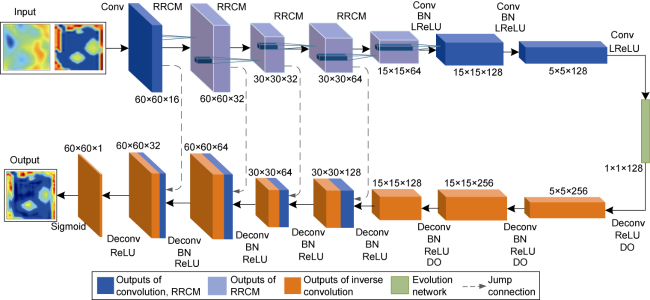
Fig. 2. The framework for the generative model in CE-GAN (the numbers indicate the dimensionality of the features computed by each layer). |
Introducing RRCMs into the coding network can enhance the feature transfer and multiplexing capabilities of the convolutional layer. As shown in Fig. 3 , the RRCM comprises multiple cyclic convolution modules with ReLU activation functions. Low-level feature information is extracted from the input reservoir performances map by means of RRCM and then residual linked with the input reservoir performances map or the reservoir performances map features obtained from shallow coding layer to get the high-level features of the multi-scale reservoir performances map, which is subsequently put into 1×1 convolutional layer for feature compression. The RRCM can effectively address the feature information and network parameter residual challenges caused by multiple convolution operations, thereby enhancing feature transfer, and making effective use of the output feature maps of each layer to improve the feature extraction capability of the generative model for reservoir performances map.
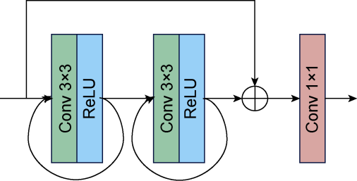
Fig. 3. The RRCM. |
In addition, the attention threshold jump connection can enhance the weight of feature information in the reservoir performances map, considering the dependence of the output reservoir performances on the input during the prediction process. As shown in Fig. 2 , threshold jump connection is used between the first four layers of the coding network and the last four layers of the decoding network to combine image feature information. It introduces the corresponding feature information of the reservoir performances map into the decoding process, providing multi-scale and multi-level fusion features for reservoir performances simulation to improve reservoir performances prediction accuracy.
2.1.2. Evolution network
The evolution network realizes potential variable evolution (Fig. 4 ) with time-varying well control as the condition, and consists of two branches. The first is a feature extractor of the potential variable ht, which is a one-dimensional CNN composed of three stacked transformed layers that using 1×5 convolution with 32, 64, and 128 convolution kernels, respectively, and a step size of 3, followed by normalization via BatchNorm and activation using the ReLU function. The second branch uses injection and production well control (the injection rate of injection well and the liquid production rate of production well), and production time as inputs, which are integrated with the features learned by the 1D CNN. The fused feature vector is transmitted to the fully connected network to predict the latent variable at the moment of t+1.

Fig. 4. The framework of the evolutionary network in CE-GAN. |
2.1.3. Framework of the discriminant model
The discriminant model is used to determine the authenticity of the reservoir performances prediction. Therefore, discriminant model D is a binary classifier capable of extraction and linear classification. It consists of a CNN with five convolutional layers (Fig. 5 ), with kernel sizes of 3×3, a step size of 2 in the first three layers, and 1 in the last two layers. The first four layers contain 32, 64, 128 and 256 convolutional kernels, respectively. Batch normalization is applied to layers 2 to 4. The LReLU activation function is used in all the layers except the first one to avoid neuron death. The inputs of the discriminant model are the actual reservoir performances maps and the simulated ones generated by the generative model. The outputs are probabilistically analyzed using the Sigmoid function and then normalized as 0 to 1, with 0 indicating false and 1 indicating true. Finally, the mean value of the output matrix is used to characterize the similarity between the simulated and the actual reservoir performances.
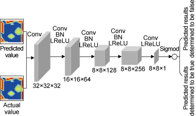
Fig. 5. The framework of the discriminative model in CE-GAN. |
2.2. Loss function considering the physical constraints
Akin to traditional GANs, CE-GAN is trained in an alternating adversarial manner, which optimizes the model parameters via alternating learning of the discriminant and generative models. Corresponding to the reservoir performances coding network, the latent variable evolution network, and the reservoir performances decoding network, we calculated reconstruction loss (Lr), evolution loss (Le), and prediction loss (Lp) of the models, which are the main components of the loss function for the generative model of CE-GAN. The computation formulas are Eqs. (6)-(8):
In addition, discriminant model D is used to distinguish between the actual data and the simulation data of generative model G and compete with G in a two-sided minimal-maximal manner. The loss function of discriminant model D is LD:
Assuming Dn(x) denotes the implicit representation of the nth layer of D, and the generative model uses average features to match with the target, the adversarial loss of the model is expressed as:
This paper also introduced a loss function based on physical constraints, i.e., the inconsistency of minimizing the fluxes between the reconstructed and predicted reservoir performances at the same time. The physical loss of flow for each producing well was defined as:
The flow rates of the producing wells located in grid j were calculated using the Peaceman model [44]:
where
When Kx=Ky, the above equation could be simplified as:
The loss function of generative model G is expressed as Eq. (13). The loss function of CE-GAN includes the loss LG from the generative model and the loss LD from the discriminant model.
3. Performance of the basic reservoir model
3.1. Dataset preparation
The performance of the reservoir performance prediction surrogate model proposed in this paper was evaluated using the classic Egg model. This model used 60×60×7 grids, 18 533 of which were active, with a grid size of 8 m×8 m×4 m. The model contained 12 wells, of which eight represented water injection wells using constant flow-rate injection, while the remaining four were constant liquid rate production wells (Fig. 6 ). This model exhibited a logarithmic permeability variance of 0.17, with correlation lengths in the x, y, and z directions of 240, 240 and 20 m, respectively. For more detailed information about this model, please refer to Reference [45].
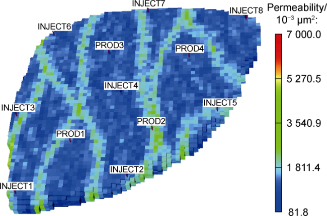
Fig. 6. The permeability and well location distribution in the Egg model (INJECT represents water injection well, PROD represents production well). |
The deterministic and stochastic Egg models consisted of 100 different permeability sets, which, along with other reservoir and fluid properties, formed the basic reservoir model used in this study. The working systems of production and water injection wells corresponding to this reservoir model were developed to simulate five years of production. The simulation times were the same for both the test and the training sets. During the simulation, the water injection and production wells were controlled by adjusting the injection and production rates over time. The well-control strategy was changed every six months, with a total of 10 control periods. The performance maps were saved at the end of each control period. Each sample consisted of the initial permeability map, the initial reservoir performance map, and the reservoir performance output maps of each control period, along with the working systems of production and water injection wells.
The control of the production and water injection wells was designed as follows. The liquid production rate of the production wells was controlled between 200 m3/d and 400 m3/d, while the injection rate of the injection wells was regulated between 120 m3/d and 180 m3/d, both of which represented continuous variables. The baseline injection rate qb for the water injection wells was randomly sampled from a uniform distribution between 140 m3/d and 160 m3/d. A random perturbation Δq was uniformly sampled in the range of [−20 m3/d, 20 m3/d]. The injection rate of the water injection wells was set as qb+Δq at each control step. There was no baseline control for the production wells. At each control step, the production rate was randomly sampled between 200 m3/d and 400 m3/d to avoid the average effect that might occur when the injection rate lacks a baseline reference, consequently increasing the oil saturation distribution. Fig. 7 shows the control programs for the water injection and production wells. Ten simulations were performed for each set of permeability, with the injection-production ratio controlled between 1.00 and 1.12 to maintain the balance between the total injection and liquid production rates. Then, 80% of the samples were randomly selected to train the neural network, while the remaining 20% were used to test the model performance.
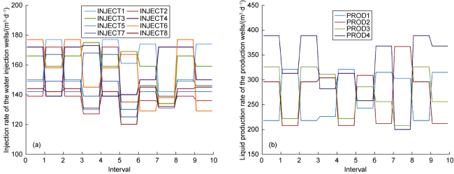
Fig. 7. The control program for the water injection wells (a) and production wells (b). |
3.2. Neural network design
The input images of the model in this paper had a vertical dimension corresponding to different layers, with an input data size of 60×60×7 and a total of 800 training samples (i.e., 80% of 100×10 training pairs). The weight coefficients of the loss function were set as follows: λ=0.01, λ1=1, λ2=λ4=0.2, λ3=0.1. Table 1 presents the key parameter settings of the model. All the network models were trained using the Adam optimizer, while decay was applied at 10 epoch intervals, with a decay rate of 0.05.
Table 1. The key parameter settings for CE-GAN |
| Parameter | Value |
|---|---|
| The latent variable dimension after encoding in the generative model. | 128 |
| The hidden layer dimension of the fully connected layer in the evolutionary network. | [64, 128] |
| The hidden layer dimension of the fully connected layer in the discriminant model. | 64 |
| The learning rates for the generator and discriminator models. | [5×10⁻⁴, 1×10⁻³] |
| Batch size. | 64 |
Since the training results were sensitive to the preprocessing methods applied to the training samples, it was necessary to select appropriate preprocessing techniques for both the pressure and oil saturation data. For the pressure data, the average value of all the data samples at each time step was first subtracted from the dataset for that step. Before training, the subsequent pressure residuals were linearly scaled to a range of [-1, 1]. After training, the data was denormalized, and then added with the average value to obtain the pressure predictions in the original domain. A residual learning method was used to preprocess the oil saturation data [46]. To prevent the oil the saturation between the adjacent steps from being too similar for the model to learn, the training target was set as the change in oil saturation . After training, the predicted oil saturation residuals were added to to generate the desired output .
3.2.1. Model performance evaluation indicators
In addition to evaluating the numerical error between the prediction results and the numerical simulation results during model testing, the Structural Similarity Index (SSIM) [47] (as shown in Eq. (14)) was used to examine the perceptual differences between the prediction results of the CE-GAN model and the numerical simulation results. The SSIM value ranged from [-1, 1], with higher values indicating a more significant degree of similarity.
3.2.2. Time and well-control data processing
Most surrogate models are not designed with sufficient consideration for the impact of the time series and can only predict production performances at fixed moments within the time range covered by the sample set, which reduces the practicality of the model. In actual applications, the working systems of the production and water injection wells continuously change over time. Therefore, the model proposed in this paper accounts for the influence of time-varying well control. It incorporates production time and well-control information as one-dimensional data to serve as the evolution control conditions for reservoir performance, which are applied to the latent features after encoding the reservoir performance.
In addition, the time and well-control data could also be transformed into a two-dimensional matrix via dimensional expansion and used as supplementary information during the training process along with the input data. The time t in the data of each sample was expanded into a matrix of the same size as the input data, with each element of the matrix representing t. In the expanded well-control data matrix, the oil and water well location elements corresponded to the production or water injection rates at the given time point, while the other positions were set to 0.
3.3. Model performance analysis
3.3.1. Model training and performance testing
To test the learning capability of CE-GAN with different amounts of training data, the CE-GAN surrogate model was trained with 200, 400, 600 and 800 training samples, respectively. Fig. 8 shows the relationship between the training loss values of CE-GAN and the number of epochs at different numbers of training samples. All CE-GAN surrogate models were trained for 1 000 epochs on nodes equipped with NVIDIA GeForce GTX 3080 GPUs. The loss values of the generative and discriminant models both stabilized after 600 epochs. The magnified view of the loss functions from 300 to 800 epochs showed that the final generative model loss converged between 0.85 and 1.06, while that of the discriminant model converged at 0.65. Compared with the generative model, the simpler structure of the discriminant model accelerated convergence.
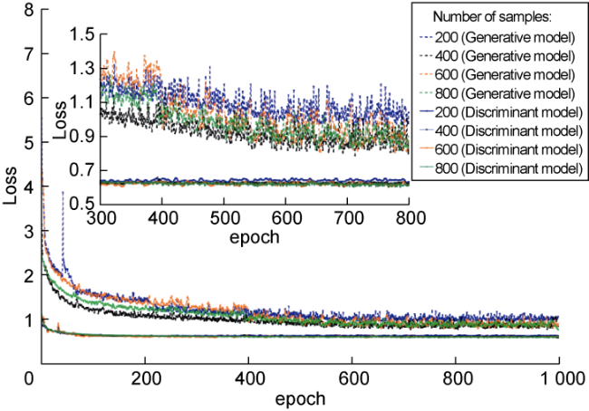
Fig. 8. The CE-GAN training loss values at different training sample sizes. |
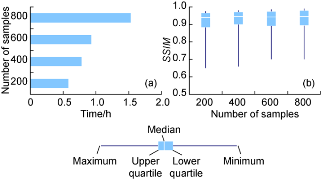
Fig. 9. The performance indicator testing of the CE-GAN surrogate model |
3.3.2. Loss function improvement
The model incorporating the physical constraint based loss function was subjected to ablation experiments. Compared with the numerically simulated pressure (Fig. 10a ), although the pressure distribution predicted by the CE-GAN surrogate model without the physical constraint loss function (Fig. 10b ) visually resembled the numerical result, the pressure residual map (Fig. 10d ) shows that the prediction results of the CE-GAN surrogate model were not consistent, particularly showing significant errors in the near-well region, which possibly have significant influence on the practical applications. Fig. 10c shows the pressure prediction results of the CE-GAN surrogate model incorporating the flow physics loss function. The maximum residual between the predicted results and the numerical simulation (Fig. 10e ) decreased from 9 kPa (Fig. 10d ) to 3 kPa. It is revealed that the accuracy and consistency of the pressure prediction results of the CE-GAN surrogate model with the flow physics loss function improve significantly, preventing unphysical local extreme values and enhancing the ability of CE-GAN to effectively perform data regression and characterize flow features.
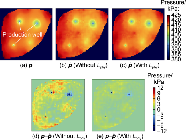
Fig. 10. The impact of physics-based loss on the pressure prediction results. |
3.3.3. Analysis of the time and well control data
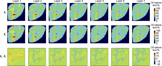
Fig. 11. The predicted oil saturation for each layer after 900 d of production with time and well control as front-end inputs of the model. |
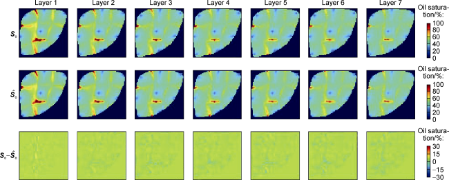
Fig. 12. The predicted oil saturation for each layer after 900 d of production with time and well control used as feature insertion in the model. |
The residuals of the predicted results were compared. Compared with the method using time and well control data as front-end inputs, the residual maps of the feature insertion method exhibited less noise and higher prediction accuracy, with the model predictions closely matching the numerical simulation results. This is because the feature insertion method can prevent the reduction in the ability to extract relevant features during the encoding process while also reducing the complexity of model training.
3.3.4. Model generalization in the time domain
After completing model training, a time-domain generalization analysis was conducted to verify the ability of CE-GAN to handle time-varying well controls. Fig. 13a and Fig. 13b show the oil saturation and pressure calculation results of the CE-GAN and numerical simulations, respectively. Columns 1 to 4 represent four different prediction time points, while rows 1 to 3 display the numerical simulation results, the predictions of the CE-GAN surrogate model, and the residuals between the two. A strong similarity was evident between the oil saturation calculated via numerical simulation and that predicted by CE-GAN. Higher relative oil saturation residuals appeared near the water injection front, with a median relative residual of 7%. The maximum relative residual (about 15%) occurred in the 360 d prediction. The pressure calculated via numerical simulation was consistent with the pressure predicted by CE-GAN, showing median and maximum relative pres-sure residuals of 0.4% and 2.0%, respectively.
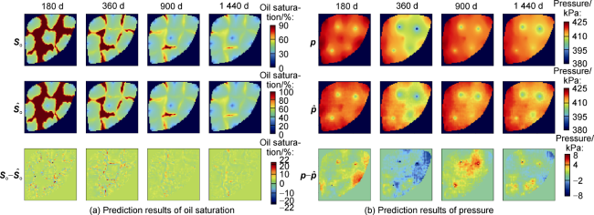
Fig. 13. The predicted pressure and oil saturation within the sample data covered time range. |
In the above case, the CE-GAN surrogate model used a dataset covering time points of 180, 360, 540, 720, 900, 1080, 1 260, 1 440, 1 520 and 1 800 d. Since the surrogate model would be required to predict continuously changing reservoir performances over time in practical applications, four time points outside the covered range (120, 450, 1 200 and 1 650 d) were selected randomly to assess its generalization performance in the time domain. Fig. 14a and Fig. 14b show the oil saturation and pressure distributions calculated by the CE-GAN surrogate model and the numerical simulation at these four time points. CE-GAN performed well in predicting the reservoir performances outside the time range covered by the training samples. The median and maximum relative oil saturation residuals were approximately 9% and 16%, respectively, while the median and maximum relative pressure residuals were 0.5% and 3.0%, respectively.
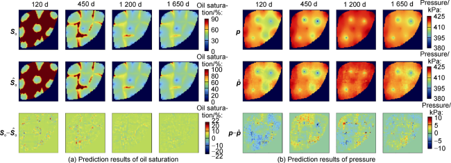
Fig. 14. The predicted pressure and oil saturation results outside the sample data covered time range. |
It is revealed that the model proposed in this paper can effectively handle time-varying well control schemes and accurately predict the reservoir performance trend over time. Although the CE-GAN surrogate model relies on numerical simulations to create sample data, its excellent generalization ability in the time domain ensures strong prediction performance. For reservoirs with similar geological characteristics and input parameter ranges (such as permeability distribution and well control) close to those of the training sample set, reservoir performance prediction can be achieved via the transfer of the reservoir performance surrogate model.
3.3.5. Model computational efficiency
The numerical simulation time was compared with the total time required for construction and prediction using the CE-GAN surrogate model. Each numerical simulation took approximately 310 s to complete a prediction. Since the CE-GAN surrogate model relied on numerical simulations to prepare training data, the time for the first 600 simulations by either the numerical simulation or the CE-GAN was the same (186 000 s). CE-GAN model training lasted about 3 380 s, equivalent to the time required for 11 numerical simulations. However, it is important to note that once training was completed, the CE-GAN surrogate model generated predictions for oil saturation and pressure at different time points and permeability distributions in only 2 s, while numerical simulations still required 310 s to run the next simulation. This represented an approximately 160-fold increase in the computational speed of the CE-GAN surrogate model.
Although the CE-GAN surrogate model requires hundreds of simulations to prepare sample data, which reduces its single-calculation efficiency, the advantage of deep learning lies in its superior generalization ability. CE-GAN demonstrates excellent prediction performance for problems requiring multiple numerical simulations. The CE-GAN surrogate model proposed in this paper is more efficient in history matching and production optimization than numerical simulations.
4. Validation of the actual reservoir model
The CE-GAN surrogate model was used for reservoir simulation in a block of the Daqing Oilfield, NW China, using 10 water injection wells and 14 production wells as the research objects. Fig. 15 shows the permeability and well-location distribution. The reservoir model contained a total of 501 768 grid cells (101×69×72), of which 389 088 were active.
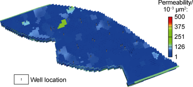
Fig. 15. The permeability and well location distribution in a block of the Daqing Oilfield. |
The simulation was performed from June 2008 to December 2018, with adjustments to the well control scheme at six-month intervals, resulting in a total of 20 injection-production control cycles. The design incorporated baseline values and sampling perturbations, with the baseline water injection rate of the injection wells ranging from 0 to 226 m3/d and the sampling perturbation ranging between −25 m3/d and 25 m3/d. A total of 200 injection-production well control simulation programs were executed, with 160 sets used for training and 40 sets for testing. All network models were trained using the Adam optimizer, with the learning rate for the generative model set to 1×10⁻⁴, while the remaining parameters following those specified in Table 1.
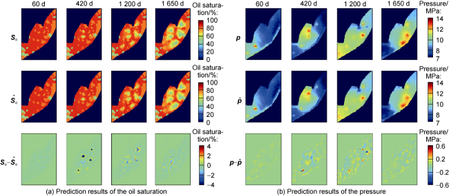
The oil saturation and pressure on June 1, 2008, were used as inputs to predict their changes over the next 10 years. Fig. 16 shows the predicted oil saturation and pressure for the eighth layer of the reservoir at 60, 420, 1200 and 1 650 d of production. The first row shows the numerical simulation results, the second row shows the CE-GAN surrogate model results, and the third row presents the residuals between the two sets of results. Both the pressure and oil saturation displayed a 4% median relative residual value, demonstrating that the proposed CE-GAN surrogate model can accurately predict reservoir performance.
Fig. 16. Change of reservoir pressure and oil saturation over time. |
Finally, the time required for numerical simulation and the CE-GAN surrogate model were compared. For the 200 test datasets, each numerical simulation run took approximately 1 920 s. CE-GAN training required about 60 556 s, which was equivalent to 31 numerical simulations. After training, the CE-GAN surrogate model took about 272 s to compute 40 test datasets, with an average prediction time of 6.8 s per case. The CE-GAN surrogate model significantly improved computational efficiency, exhibiting a speed increase of almost 280-fold compared with previous methods. Therefore, if more than 231 simulations are required during production optimization, the CE-GAN surrogate model should be used to simulate reservoir development behavior in actual conditions. This approach facilitates reproducible, highly efficient development plan design, evaluation, selection, and optimization.
5. Conclusions
This study proposes an innovative reservoir performance prediction surrogate model based on CE-GAN, defining the reservoir performance prediction problem in the manifold space and transforming it into an image-to-image regression problem. The surrogate model uses permeability distribution, initial reservoir performance, and time-varying well control as inputs. Production time is treated as an additional input to the network, enhancing the generalization ability of the model in the time domain. Additionally, a training strategy combining regression loss and physics-based loss is introduced, allowing the model to better approximate the discontinuous distribution of reservoir performance. Ultimately, this enables the rapid prediction of reservoir performance under time-varying well control.
The performance of both the basic reservoir model and the actual reservoir model is validated. The CE-GAN- based reservoir performance prediction surrogate model successfully accounts for the impact of reservoir heterogeneity and well control changes on reservoir performances. It accurately predicts approximate pressure and oil saturation values in waterflooding reservoirs under time-varying well control. Moreover, the model can describe reservoir performance at any given time with precision. Although preparing the deep learning sample dataset requires a significant amount of time, the prediction efficiency of the model is approximately two orders of magnitude higher than traditional numerical simulations, making it a suitable replacement for handling computationally intensive tasks such as history matching and production optimization.
Acknowledgments
We appreciate the Exploration and Development Research Institute of PetroChina Daqing Oilfield Co. Ltd. for providing the oilfield production data.
Nomenclature
ct—reservoir performance evolution conditions for all grids at time t;
c1, c2—constant;
C—forcing term;
d—grid height, m;
Dn(x)—the implicit representation of the nth layer in the model D;
E—expectation function;
—reservoir performance prediction surrogate model;
F()—model operator;
Gdec,θ—decoding network, where θ represents the model parameters of the decoding network;
Genc,ϕ—coding network, where ϕ represents the model parameters of the coding network;
Gevo,ψ—evolution network, where ψ represents the model parameters of the evolution network;
ht—the latent variable at time t encoded from xt;
ht+1—the latent variable at time t+1 encoded from xt+1;
—the latent variable at time t+1 evolved from ht;
K—permeability, m2;
Kj—the permeability of grid block j, m2;
—the relative permeability of phase l in grid block j at water saturation Sw, dimensionless;
Kx, Ky—permeability in the x and y directions, m2;
Ladv—the adversarial loss of the generative model G;
Le—evolution loss;
LD—the loss value of the discriminant model D;
LG—the loss value of the generative model G;
Lp—prediction loss;
Lphy—physical constraint loss;
Lr—reconstruction loss;
nb—number of grids;
nh—the dimension of the latent variable;
nw—number of wells;
—pressure predicted by the CE-GAN surrogate model, Pa;
pj—grid pressure of grid block j, Pa;
pt—pressure of all grids at time t, Pa;
pw—bottom hole flowing pressure, Pa;
Δq—random perturbation of the water injection rate, m3/d;
qb—baseline water injection rate, m3/d;
—flow rate of phase l in grid block j, m3/s;
qw,t—actually monitored well flow rate at time t, m3/d;
—well flow rate at time t predicted by the CE-GAN surrogate model, m3/d;
ro—equivalent radius, m;
rw—wellbore radius, m;
, , —nb, nh, and nw-dimensional vector spaces over the real number field;
SSIM—structural Similarity Index, dimensionless;
—oil saturation predicted by the CE-GAN surrogate model, %;
—oil saturation at time t, %;
St—oil saturation of all grids at time t, %;
Sw,j—water saturation of grid block j, %;
t—time, d;
Δt—production time, d;
x, y, z—the three directions of the reservoir;
Δx—grid length, m;
xt, xt+1—the reservoir performance assemblage for all grids at times t and t+1;
—the reconstructed state obtained without latent variable evolution;
—the reservoir performance prediction map at time t+1 obtained by decoding the latent variable ;
X—reservoir performance;
Δy—grid width, m;
γ—network parameters;
ξ—boundary and initial conditions;
λ—flow physics loss adjustment weight, dimensionless;
λ1—adversarial loss adjustment weight, dimensionless;
λ2—reconstruction loss adjustment weight, dimensionless;
λ3—evolution loss adjustment weight, dimensionless;
λ4—prediction loss adjustment weight, dimensionless;
μl—viscosity of fluid l, Pa•s;
μu, μv—the mean of images u and v;
σu, σv—the variance of images u and v;
σuv—the covariance of images u and v, dimensionless;
Λ—geological model parameters.