

Introduction
Imaging techniques, such as Computed Tomography (CT), can be utilised to capture the internal structure of porous media, including rocks, membranes and biological tissues. The acquired images are commonly segmented into pore and solid components and are used in processing and simulation workflows to determine petrophysical, mechanical, electrical, and flow properties of the media [1]. In this context, deep learning can leverage existing data to establish a more favourable balance between the accuracy and scalability achieved, and the time and money expended. However, the prediction of pore-scale multiphase flow using deep learning has remained elusive. In this work, we address this challenge by creating two-phase drainage models that are faster and cheaper than simulations and experiments.
Deep neural networks (DNNs) are forms of artificial neural networks that contain many layers and are trained on large datasets [2]. They have found numerous applications in geosciences [3-4], including image super-resolution [5], segmentation [6], and permeability prediction [7]. Considering single-phase flow fields, DNNs have been primarily applied to estimate pressure and velocity fields. Santos et al. [8] implemented a U-Net-based Convolutional Neural Network (CNN) to determine 3D fluid velocity fields much faster than the Lattice Boltzmann Method (LBM) [9]. Kamrava et al. [10] captured the dynamic nature of flow by modelling pressure and velocity fields in porous membranes at four times using a recurrent architecture. Deep learning can also be integrated with full-physics simulations to set the initial conditions for faster convergence [11], compress and accelerate simulation steps [12], or complete a cumbersome part of a procedure in a shorter time period [13].
Deep learning research on multiphase flow in microstructures has been rather scarce. Rabbani et al. trained a CNN to predict two-phase relative permeability and Leverett J-function in semi-real 3D volumes [14]. Feng and Huang devised a CNN to estimate 2D pressure and saturation fields at breakthrough time [15]. Wang et al. formulated a conditional Generative Adversarial Network (GAN) to realize distributions of fluids during drainage under low capillary numbers [16]. Yu et al. trained an attention U-Net to predict saturation and pressure fields at 0.8 ms during water invasion in gas-occupied media [17]. The foremost challenge lies in applying these models to complex pore geometries. Studies typically consider simplified porous media that are limited in variety and realism. Furthermore, they seldom incorporate resolution and descriptors of rock and fluid interactions alongside images. The same is true for displacement parameters, leading to models that lack pressure or rate sensitivity.
In this study, we concentrate on the pore-scale estimation of two-phase, capillary-dominated primary drainage in realistic rock-fluid systems. During drainage, a rock initially saturated with a Wetting Phase (WP) is subjected to Non-Wetting Phase (NWP) invasion at multiple equilibrated pressure steps. We train a deep neural network to predict the simulated fluid distribution image at each capillary pressure (pc) directly from pore-solid images across a range of pixel sizes (Sp), interfacial tensions (σ) and contact angles (θ). This task entails classifying pixels as displaced and non-displaced while honoring (1) local fluid-fluid and rock-fluid interactions and (2) NWP connectivity to the inlet across spatial and temporal (pc steps) dimensions.
We call Sp, σ, θ, and pc scalar features and consider them as inputs, distinguishing our research from related work. This study presents multiple other novelties. First, we build a diverse dataset of unprecedented size. Second, we avoid complex feature engineering, leading to general end-to-end models. Third, we explore three vastly different DNNs and compare their strengths and limitations. Fourth, we introduce an effective strategy for size-agnostic predictions on any inlet-outlet setup, rendering the final model multiscale and multi-boundary.
1. Dataset development
To generate a pore-solid (binary) image dataset, we collect 20 segmented 3D micro-CT scanning images, covering pores and solid particles of different sizes and shapes. The images consist of one synthetic silica sample (3003), nine sandstones (3003), one Berea sandstone (4003), two carbonate rocks (4003), one sand pack (4502×425), five other sand packs (4503) [21-22], and one random packing of sphere (5003) [23].
These parent cubes are sliced along X, Y and Z axes. These slices are cropped into randomly positioned rectangular regions, with their sides separately determined from a normal distribution with a mean of 128 and a standard deviation of 24. The rectangles are then resized to 1282. Fig. 1 illustrates the porosity histogram and ten example subsamples from each rock type. Sandstones and carbonates show the greatest intra-type diversity.
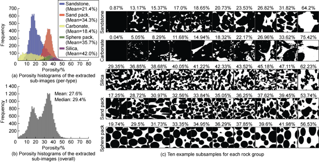
Fig. 1. Porosity histograms and example subsamples for each rock type (in Fig. (c), percentage represents porosity, and white and black zones represent pore and solid pixels). |
We augment the dataset by applying seven affine transformations: rotations of 90°, 180°, and 270°; horizontal and vertical flipping; and horizontal and vertical flipping, each followed by a rotation of 90°. This produces a total of 177 360 subsamples. To create a holdout testing dataset not seen during training, we extract the central sub-images (sized 1282) from five equidistant slices along the Z-axis of each of the twenty parent rocks. After excluding samples with no pores connected to the inlet, 97 testing images are obtained.
Two-phase flow through porous media can be modelled by a variety of methods, including Pore Network Modelling (PNM) [24], Pore-Morphology-based Simulation (PMS) [25-26], and LBM [9]. PMS is computationally much lighter and can be directly applied to any given binary structure. It is well established that it can produce comparable results to experimental observations, PNM and LBM when simulating two-phase fluid displacement, even though it may neglect some physical phenomena (such as phase trapping) [25⇓-27].
Hilpert and Miller [25] devised PMS to simulate quasi-static primary drainage in totally wet porous media. The method is typically formulated by a series of morphological erosions and dilations. PMS was later extended to partially wet porous media with a constant contact angle [28] and a locally variable contact angle [29]. This is achieved by rescaling the erosion diameter with a factor of cosθ, where θ is limited within [0°, 60°] to minimize artefacts and over-prediction of the NWP saturation. We implement Schulz's algorithm [29] via exact Euclidean distance transformation, which is faster and more precise than morphological operations.
It is assumed that a binary porous medium (Fig. 2a ) is connected to NWP reservoir on the left (inlet) and to WP reservoir on the right (outlet), and all boundaries except inlet and outlet are sealed (i.e., impermeable). The Euclidean distance from each pore point (pixel or voxel) to the nearest solid point is calculated, and thus a Distance Map (DM) is obtained (Fig. 2b ). Then the calculations are carried out via the following steps:
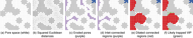
Fig. 2. Distance-based PMS implementation (grey represents rock pixels, and blue represents the pore region isolated from the inlet). |
(1) At each pc increment, two radii, r=2σ/pc and r°=rcosθ are calculated.
(2) The pore space is eroded (purple regions in Fig. 2c ) by removing all pore points with DM£r°. The blue region in the figure is isolated and will not be displaced.
(3) The eroded pore regions that are not connected to the NWP reservoir are discarded, determining the remaining eroded pore regions that are connected to the inlet (purple regions in Fig. 2d ).
(4) A new distance map, DM°, calculates the shortened distance from every pore point to the remaining regions (purple regions in Fig. 2d ). When calculating DM°, the points in the remaining regions are assigned zero values. Also, the solid points are assigned infinity to avoid NWP invading the solid areas.
(5) All the pore points with a DM°£r are combined with the remaining regions into larger spaces, forming newly dilated areas invaded by NWP (red areas in Fig. 2e ). The green regions in Fig. 2f could be considered trapped; otherwise, they will all be invaded at higher pc.
(6) The above steps are repeated for the next pc (smaller radius) until a stopping criterion is satisfied.
We apply PMS to WP-saturated images that are connected to an NWP reservoir on the top (inlet) and a WP reservoir on the bottom (outlet). Drainage is simulated until full desaturation, under the assumption of film/corner flow. We perform three simulations per image, each with logarithmically spaced pc (Pa) steps and scalar features randomly selected from these uniform distributions: Sp: [1 μm, 50 μm], θ: [0o, 60o], σ: [0.015 N/m,0.065 N/m]. The fluid distribution corresponding to each lgpc in each simulation is recorded.
Following simulations, we transform pore-solid images into exact Euclidean distance maps and normalize them by the maximal distance across all samples. We also log-transform pc and apply min-max normalization to all scalar features. We randomly select the maximum number of simulation data points that result in a roughly uniform saturation distribution. Finally, we binarise phase distributions so that one indicates NWP and zero signifies WP and solid. This reduces the problem to a pixel-wise binary classification. Therefore, predictions will be probability maps of invasion, which we ultimately binarise by Otsu thresholding.
2. Model development and analysis
In this section, we train and evaluate convolutional, recurrent, and transformer networks to predict fluid distributions. Fig. 3a provides an overview of the training process using PMS simulation results. Black, grey, and white indicate solid, WP, and NWP, respectively. Models consider the distance map and the scalar features as inputs. All training is performed in 32-bit precision mode on an Nvidia RTX 3080 GPU (16GB) using a Binary Cross-Entropy (BCE) loss function and an Adam optimiser [30]. Fig. 3b depicts how a trained model can be used to develop drainage results for a new rock-fluid system at consecutive pressures.
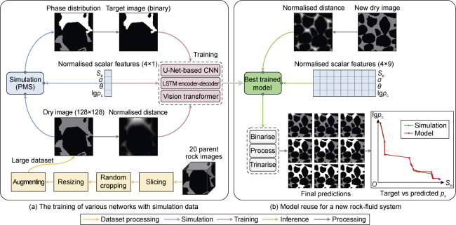
Fig. 3. Network training based on PMS simulation results and application of the model to a new rock-fluid system (black, gray and white represent solid, WP and NWP, respectively). |
2.1. U-Net-based CNN
We first explore CNNs to directly predict phase distributions from the inputs. Here, we consider the data from the sphere pack, comprising 732 772 phase distributions. This is because most real 2D samples are not hydraulically connected from top to bottom. Following data selection for a uniform saturation distribution, we are left with 261 618 instances for model training (90%) and validation (10%).
2.1.1. Architecture and training
The U-Net CNN has consistently proven successful in related image-to-image applications [4,31]. We, therefore, start by adapting this architecture to our problem. Since U-Net only takes images as inputs, we add a new input branch that upsamples the scalar features through multiple dense layers and a reshape layer. The result is concatenated with the output of the contracting path at the bottom of the network [31], resulting in a Y-like structure. The network, which we call Y-Net, uses Leaky ReLU activations in its hidden layers and culminates in an output layer with a single Sigmoid-activated kernel. We train Y-Net for 20 epochs with an initial learning rate of 0.000 5 and a batch size of 64, taking 93 minutes per epoch.
2.1.2. Testing
We evaluate the Y-Net against 222 unseen testing instances from the sphere pack. This results in F1 Score, Intersection Over Union (IOU), Mean Square Error (MSE) and NWP saturation correlation coefficient (SnwR) values of 0.938 0, 0.880 6, 0.017 8, 0.956 9, respectively. These suggest high pixel-wise accuracy in spite of a certain degree of overfitting. Overall, Y-Net can simulate the process of WP displacement from pores in the right pc ranges, as evidenced by a high SnwR. In addition, Y-Net is very fast, taking only 0.065 s to yield one fluid distribution.
However, Y-Net occasionally results in three kinds of errors: (1) disconnected invading phase; (2) jagged or pixelated fluid-fluid interface; and (3) ending the displacement inside a pore rather than at the throats. Fig. 4 shows the worst-case mistake made by Y-Net for the sphere pack and other rock types. Most errors are associated with the model's failure to establish NWP connectivity. As shown for one example in Fig. 4b , the network ultimately generates the correct phase distribution at pi+1 but it does not follow a physical and continuous displacement path from the inlet as observed at pi.
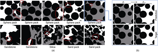
Fig. 4. The worst-case prediction mistakes made by Y-Net. |
The root reasons for the above-mentioned prediction mistakes lie in two inadequacies of the Y-Net. First, neither the input data nor the loss function promotes the neural network to learn about the characteristics of fluid connectivity or the role of throats as displacement bottlenecks. Second, CNNs are adept at detecting local and hierarchical features, but they lack sensitivity to global patterns and long-range relationships, which are the essence of inter-pore fluid connectivity [32]. Therefore, although Y-Net can be architecturally improved [15,17], this alone could not resolve the underlying limitations of this model.
2.2. Convolutional LSTM encoder-decoder
It is possible to incentivize the model to uphold NWP connectivity by allowing it to look at the phase distributions in preceding rows as a reference. To facilitate this, we sequence images along the fluid invasion direction from inlet to outlet, i.e., from top to bottom along the Y-axis, creating a new dataset of consecutive and overlapping windows instead of single images. The window is a sequence data unit, whose size (thickness) is a key hyperparameter. A sequence model develops memory by analyzing the rows inside each window one by one. A trained model is able to carry out autoregressive predictions by reusing its own previous prediction (fluid distribution in the former window) along with the new inputs of the current window (distance map and scalar features) to predict the fluid distribution in the current window, potentially leading to a smooth and valid displacement.
Similar to Y-Net, we train with the sphere pack subsamples. We find that a window size of 32 optimally balances performance and computational cost. Windowing with this size and a stride of one result in 1.4 million windows, half of which is used for training (90%) and validation (10%).
2.2.1. Architecture and training
Recurrent Neural Networks (RNNs) allow circular connections where each output can affect the next predictions, enabling them to efficiently work with sequential data of arbitrary lengths [33]. However, classic RNNs tend to lose accuracy for longer sequences. To recognize long-term dependencies, the Long Short-Term Memory (LSTM) cell has been introduced [34]. In this study, we use the encoder-decoder RNN [35] with convolutional bidirectional LSTM cells. Encoder-decoder has been a popular choice for sequence-to-sequence problems such as neural machine translation, where each word is translated based on the context of the surrounding words. This context is conceptually similar to the global phase connectivity.
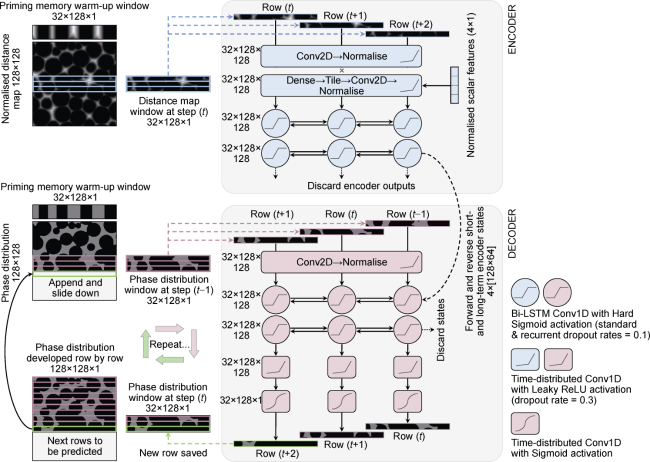
Fig. 5. Architecture of convolutional LSTM encoder-decoder (the size of the window for autoregressive prediction is 32). For visual clarity, a window size of 3 is assumed here. |
We name this model Ψ-Net, reflecting its structure with three inputs and one output. We train Ψ-Net with a batch size of 32 and an initial learning rate of 0.001 in ten epochs, averaging 764 minutes per epoch.
2.2.2. Testing
We evaluate Ψ-Net on the same 222 unseen sphere pack samples as Y-Net, resulting in F1 Score, IOU, MSE, and SnwR of 0.920 4, 0.853 1, 0.027 3, and 0.934 4, respectively. Fig. 6 plots the target and predicted invading phase distributions for three unseen samples. Warmer colours represent earlier stages of displacement, and cooler colours represent later ones. For each sample, the figure also includes the targets and predictions for two steps of interest. Overall, the results are satisfactory. Although the pixel-wise match is higher for Y-Net, Ψ-Net proves much more capable of meeting the physical connectivity requirements.
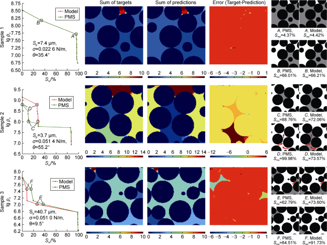
Fig. 6. Ψ-Net performance on three testing samples from the sphere pack (warm colours represent earlier stages of displacement, and cool colours represent later ones.) |
During long autoregressive predictions, performance may gradually decline as errors pile up. Fig. 7 investigates the moving averages of three metrics across all rows of the samples in Fig. 6 . The figure and our visual evaluations confirm that there is no evidence of error build-up in rows closer to the outlet.
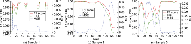
Fig. 7. Moving averages of performance metrics for all rows of the three samples from |
On the other hand, Ψ-Net appears to be prone to directional bias, which encapsulates the model's tendency to perform best when the invading fluid moves downward in the same direction data are sequenced. Sample 2 in Fig. 6 showcases one example, as marked by arrows, where this has set the predictions back multiple steps. Despite this, the model eventually recreates all non- downward patterns at higher pressures. On rare occasions, Ψ-Net may even invade pores through non-downward flows earlier than the simulations (see Sample 3 in Fig. 6 ). Aside from this, sequence models are slow to train, and autoregressive inference is time-consuming. Ψ-Net takes an average of 2.898 s to generate one phase distribution. In the next section, we train a network that is statistically more accurate than Y-Net and physically sounder than Ψ-Net.
2.3. Vision transformer with higher-dimensional data
If there were no order to pores and all were revealed to the NWP reservoir from the outset, drainage would happen based solely on pore sizes. This would render each pore independent, thus negating inter-pore connectivity. To make this possible, we modify our simulator to skip step 3, where the inlet-isolated eroded sub-spaces are discarded. The outcome is equivalent to running 3D simulations on 2D rocks along the Z-axis, i.e., along a higher dimension. Once the model generates predictions, we impose any desired inlet-outlet setup by excluding displaced regions that are not connected to the inlet(s).
Since this approach does not require end-to-end hydraulic connectivity, we run higher-dimensional simulations on sub-images of all parent rocks. Selection for a uniform saturation distribution leads to a final set of 9 551 504 instances for training (97%) and validation (3%).
2.3.1. Architecture and training
Vaswani et al. [36] introduced an efficient encoder-decoder architecture called a transformer, which captures pairwise relevancies in sequences by attention mechanisms. This mechanism can also operate in a self-mode to grasp relations within one sequence. To apply self-attention to images, the Vision Transformer (ViT) was proposed [37]. Contrary to CNNs, ViTs do not have a locally restricted receptive field and can capture long-range dependencies. Paul and Chen [38] provide empirical evidence on how ViTs can be more robust than CNNs.
Our modified ViT implementation is illustrated in Fig. 8 . First, distance maps are broken into 16×16 (N=256) non-overlapping patches of size 8×8. The patches are flattened and embedded into 128-dimensional spaces (256×128). All transformer layers will use tensors , where N and D are the sequence length and the embedding dimension of the model, respectively. To add knowledge of patch orders, a vector of integers is created and linearly projected to the same size. Scalar features are also processed into this size through a pair of dense layers and a reshape layer. We add together patch, position, and scalar embeddings to develop a combined representation for the transformer encoder.
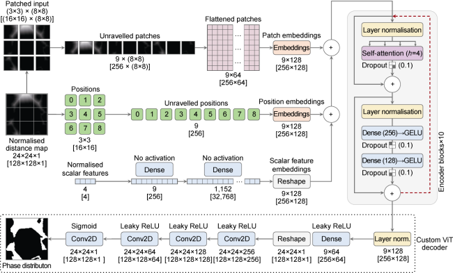
Fig. 8. ViT architecture. An input image size of 24×24×1 is assumed for enhanced readability. True sizes are shown in brackets. |
Our transformer consists of ten stacked blocks, each with a Multiheaded Self-Attention (MSA) module and a feed-forward one. In basic self-attention, Z is transformed into three matrices of queries (Q), keys (K), and values (V), which are used to calculate the attention score by the scaled dot-product mechanism shown in Eq. (1), where d is the dimension of the key vector. The multiheaded approach runs h self-attentions in parallel, called heads. The results are concatenated and linearly projected to produce the final output. The MSA in our model has four heads. Also, the feed-forward module has two dense layers with GELU activations [39].
The encoder output is passed to a custom convolutional decoder, which generates the phase distributions. By incorporating a decoder CNN, we build some level of spatial inductive bias (e.g., locality and translation equivariance) into the architecture, making it better poised to recognise both global and local patterns.
We train the ViT with Higher-Dimensional data (HD-ViT) using a batch size of 64 and an initial learning rate of 0.000 5. Training is concluded after eight epochs, each taking a little over 13.5 hours.
2.3.2. Testing
We test HD-ViT by creating a separate dataset of 6 323 higher-dimensional phase distributions from all parent rocks. Fig. 9 shows PMS and HD-ViT fluid distributions in different types of rocks. The testing F1 Score, IOU, MSE and SnwR are 0.962 5, 0.927 0, 0.003 9 and 0.966 5, respectively, indicating excellent performance, which also consistent for all rock types. HD-ViT generates each fluid distribution in just 0.037 s, which is two orders of magnitude faster than Ψ-Net and about two times the speed of Y-Net, demonstrating its very high efficiency. Importantly, HD-ViT ensures NWP connectivity in the entire process of invasion. Moreover, several fluid distributions can be generated from each higher-dimensional prediction by taking different sides of sample as inlet (multi- boundary feature).
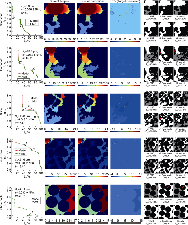
Fig. 9. HD-ViT targets and predictions for five testing samples (warm colours represent earlier stages of displacement, and cool colours represent later ones). |
3. Model verification and extension to 3D
3.1. Performance vs rock type and image size
To verify the multiscale capabilities of HD-ViT over various rock types, we obtain new 3D segmented micro- CT scans as parent rocks: two sandstones (Bentheimer and Doddington) and two carbonates (Estaillades and Ketton), all sized 10003, with porosity values of 21.7%, 19.6%, 12.7%, and 13.3%, respectively [40-41]; and a new sphere pack of size 9003 with porosity of 36.9% [42].
For each image, we extract randomly positioned equilateral 2D sub-images from all slices along the three axes. We then remove subsamples that are not hydraulically connected from one end to the opposite end. After augmentation (180° rotation and horizontal/vertical flipping), we conduct three simulations per image. Finally, a maximum of 100 simulations are chosen at random. This process is repeated for side lengths from 1002 up to 10002. To predict on larger images, distance maps are zero-padded and broken into overlapping patches of size 1282 with a stride of 64. Outputs are then cropped by half of the overlap and stitched back together to reconstruct the full image. Fig. 10 depicts three example predictions on large images. While HD-ViT might be slightly early or late in prediction at certain capillary pressures, it seldom mistakes the displacement order of pores (see the 37th pressure step in the Ketton rock in Fig. 10 ).
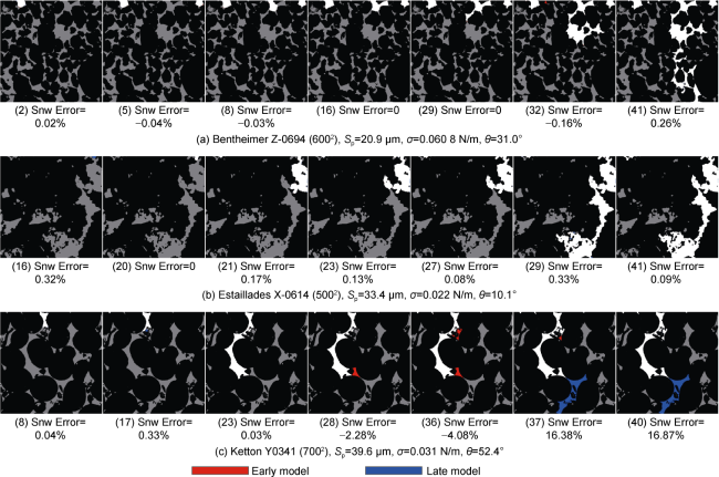
Fig. 10. HD-ViT predictions for three new larger images (the numbers in bracket represent the series number of pressure step). |
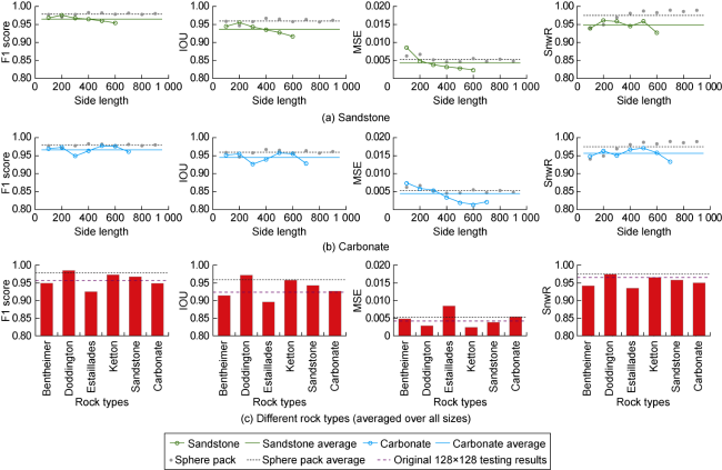
Fig. 11. HD-ViT performance vs. rock type and image size. |
3.2. Model runtimes compared to simulations
We compare the average wall-clock runtimes of HD-ViT and PMS for one phase distribution. Fig. 12a shows the relationship of runtime vs. patching stride and image size. As expected, with larger strides, HD-ViT runs relatively faster. Due to the patch overlaps, the network is effectively predicting more pixels than PMS. For an equitable comparison, in Fig. 12b we plot runtimes against the actual number of pixels processed, showing linear relationships. HD-ViT is initially slower than PMS but overtakes it at some critical size. Next, we utilize the linear relationships and extend and plot runtimes vs. original image pixel counts for different strides. Fig. 12c presents the intersection points between the HD-ViT runtime trendlines and the PMS trendline. These points translate into critical sizes of 509.02, 692.92, 1051.02, and none (no meaningful intersection), for strides of 128, 112, 96, and 64, respectively.
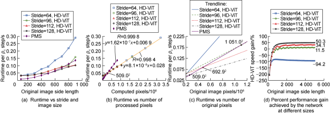
Fig. 12. Runtime comparison between HD-ViT and PMS. |
Given runtimes follow a linear trend, their ratio converges to a constant value in sufficiently large images. This ratio represents the ultimate speed gain achieved by HD-ViT over PMS. As shown in Fig. 12d , the stride of 64 increases the runtime by 94.2%, while strides of 96, 112, and 128 decrease runtime by 11.5%, 34.1%, and 50.3%, respectively. To balance performance and runtime we select the stride of 112 as the optimal choice, corresponding to 34.1% speed gain.
3.3. Experimental verification
As shown in Fig. 13a , McClure et al. [43] injected nitrogen (NWP) into a decane-saturated (WP) 2D microfluidic device and captured fluid distribution images at different pressures. They then introduced an averaging method to approximate the microscale pc. The method relies on interfacial curvatures and accurate pressure fields from LBM simulations initialised using experimental fluid distribution images (called LBM-E here). They also ran simulations initialized with random phase distributions (LBM-R) to establish the full range of fluid saturations.
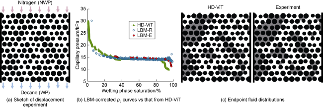
Fig. 13. Comparison between HD-ViT, experiments, and LBM simulations in a 2D micromodel. |
We use HD-ViT to make predictions with the same σ (24.7 mN/m), θ (4.1°) and pressure range as those in McClure et al. [43]. Fig. 13b shows the resulting pc curves, indicating that HD-ViT can reproduce the pressure-saturation relationship, particularly the region where the bulk of decane desaturation occurs (saturation ranging from 20% to 90%). The small discrepancies between HD-ViT and LBM curves have most likely occurred because of the inherent differences between the two techniques. The difference between LBM-R and HD-ViT at high WP saturation may be caused by the randomness of LBM-R (LBM-R and LBM-E are not completely matched themselves).
To compare fluid distributions, we correct HD-ViT results by tracking the connectivity of WP to the outlet, so as to account for irreducible WP saturation. If any WP-filled region becomes disconnected from the WP reservoir at a certain pressure, we disallow NWP to invade it in subsequent steps. The ultimately predicted endpoint phase distribution closely matches the physical experimental image, presented in Fig. 13c . The data shown in Fig. 13 uses the prediction results from HD-ViT for over 1 000 pressure steps, which took just about one minute.
3.4. Extension to 3D
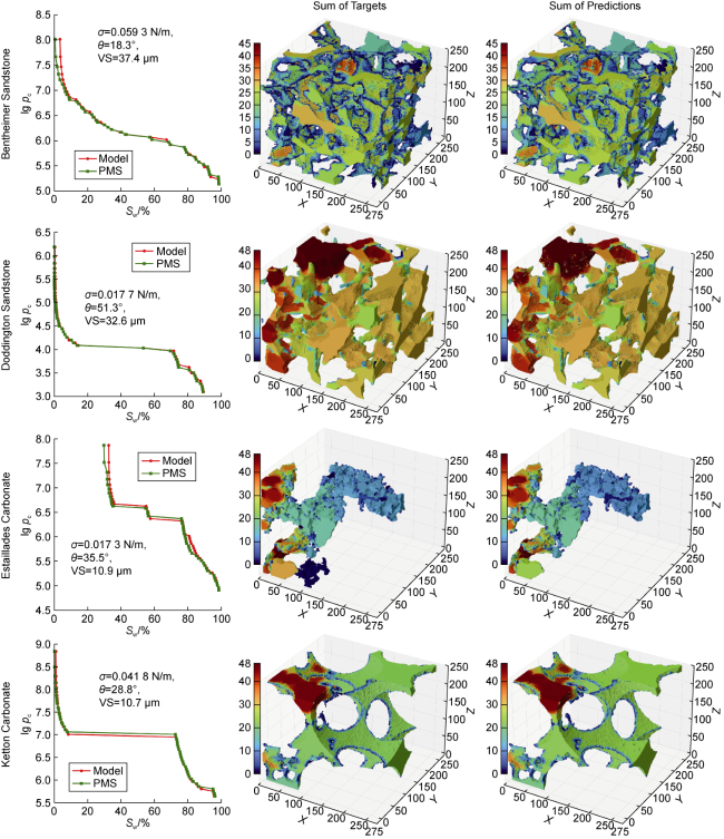
It is worthwhile to examine whether HD-ViT can be feasibly applied to 3D domains (using 3D input and output images) with minimal alterations. We create a 3D dataset by decomposing each of the twenty parent rock images into overlapping cubes of size 643. Simulation and selection for a uniform saturation distribution result in 367 842 instances. To develop a testing dataset, we take one central cube of size 2563 from each of the new 3D rock images (Bentheimer, Doddington, Estaillades and Ketton), producing 696 fluid distributions.
Two changes are necessary to repurpose HD-ViT for 3D: (1) the transformer input ( ) should result from an input volume, and (2) the decoder must be a 3D CNN. The latter is straightforward, and the former can be accomplished with tubelet embedding, which is used to tokenise videos in Video Vision Transformer (ViViT) [44]. In our adaptation, named HD-ViViT, we divide each 3D image into 512 (N) non-overlapping 3D sub-volumes of size 83. These are then flattened and linearly projected with an embedding dimension of 256 (D). A vector of integers in the range and the scalar features are also embedded with the same size (512×256). The model is trained for six epochs (9.5 hours per epoch) with an initial learning rate of 0.000 5.
The testing F1 Score, IOU, MSE, and SnwR for samples sized 2563 are 0.968 4, 0.944 0, 0.003 6, and 0.989 5, respectively. Fig. 14 compares PMS targets and HD-ViViT prediction results for one simulation from each testing rock type. HD-ViViT successfully reproduces the distribution of the invading fluid in various rock types. The results highlight the immense potential of transformer-based models to capture pore-scale 3D flow.
Fig. 14. pc curves and fluid distributions of four testing rocks by PMS simulation and HD-ViViT prediction (warm colours represent earlier stages of displacement, and cool colours represent later ones). VS stands for Voxel Size. |
4. Conclusions
We developed an accurate vision transformer (HD-ViT) to predict the distribution of fluids during two-phase capillary-dominated drainage from pore-solid images, considering a wide range of pressure and rock-fluid properties. The network was trained on a large and diverse dataset generated by our Pore-Morphology-based Simulator (PMS). We validated the model by achieving excellent performance on larger images of unseen sandstone and carbonate rocks. We demonstrated the speed advantage of HD-ViT by reproducing the LBM-derived pc curves and experimental phase distributions from a microfluidic drainage test. Finally, a feasibility study revealed that the same methodology can successfully be extended to 3D porous media.
The trained models can be used to replace slow direct simulations or lengthy experiments, given a tolerance for accuracy. They could also be employed to generate finer steps between available points or validate other results. Additionally, models may be fine-tuned for higher-quality, computationally intensive, or domain-specific datasets with limited instances. Predictions could also be used as initial conditions to expedite direct simulations. Due to their speed, it is possible to integrate models into other workflows as fast predictors, e.g., uncertainty/sensitivity analysis and inverse problems. More importantly, the scalability of the transformer-based models and the multiscale processing capabilities of the higher-dimensional approach enable distributed computing for large images (10003 and above). As such, the methodology proposed in this paper can be a powerful solution to the limitations regarding image size, dataset size, and computation capacity. The major next steps for this research are advancing the 3D modelling, adding greater diversity to the inputs, and modelling imbibition and dynamic displacement.
Acknowledgements
We would like to extend our gratitude to Prof Vasily Demyanov, Dr Jim Buckman, and Prof Kenneth Sorbie for their thoughtful contributions. We thank the High-Performance Computing Platform of the Southwest Petroleum University of China for supporting this work. This research forms a component of a PhD study, which has been made possible through a James Watt Scholarship offered by Heriot-Watt University. This paper has also been supported by the International Cooperation Programme of Chengdu City (No. 2020-GH02-00023-HZ).
Nomenclature
D—embedding dimension of HD-ViT;
d—dimension of the key vector;
h—number of self-attention heads;
N—sequence length;
pc—capillary pressure, Pa;
pi, pi+1—capillary pressures at steps i and i+1, Pa;
Q, K, V—matrixes of queries, keys, and values;
—real number space;
Sp—pixel size, μm;
Sw—wetting phase saturation, %;
Snw—non-wetting phase saturation, %;
t—row number;
X, Y, Z—Cartesian coordinate system;
Z—input tensor to transformer;
σ—interfacial tension, N/m;
θ—contact angle, (°).