

Introduction
Screening techno-economic factors is important for efficient shale gas development [1⇓⇓⇓⇓⇓⇓⇓⇓⇓⇓⇓⇓⇓-15]. Common conventional screening methods include 3D seismic data interpretation, logging data interpretation, full data utilization, multi-data integration, and analogical study [16⇓⇓⇓⇓⇓⇓⇓⇓⇓-26]. Ma et al. [27] and Altamar et al. [28] evaluated and analyzed potential shale gas resources in China by categorizing key geological, engineering and economic indicators. Li et al.[29] used superimposed maps of key parameters to discern the distribution of shale gas sweet spot zones. In addition to common evaluation indicators [30], Jing et al.[31] suggested that the structural characteristics and locations of shale gas reservoirs also play an important role in sweet spot identification. However, these methods above suffer from inconsistent selection of parameters. In terms of economic evaluation of shale gas, Madani et al.[32] used economically and technically recoverable reserves to discriminate the sweet spot zone. However, such a multi-parameter evaluation method has not been applied in screening traditional sweet spot zones, especially in undeveloped regions.
This paper proposes a systematic stepwise approach which integrates technical indicators, such as TOC and Ro, and economic ones, such as internal rate of return (IRR) and payback period, for discriminating the most favorable zones in unexplored prospects, and selects the Lurestan shale gas area in Iran as a case to study how to reduce development risks and achieve effective and economic production of shale gas.
1. Techno-economic assessment of shale gas
The method used in this paper to distinguish the best techno-economic shale gas zones is summarized as the following four steps: (1) identification of geological sweet spot zones; (2) analogy study of key development parameters; (3) estimation of technically recoverable reserves and wells required to completely cover the sweet spot zones; (4) economic evaluation of geological sweet spots.
1.1. Key parameters for identifying geological sweet spot zones
The potential of shale gas is influenced by multiple factors, of which key parameters include H, TOC, Ro, Gc, mineral content, reservoir depth, porosity, permeability, and mechanical properties [33⇓⇓⇓-37]. Geological sweet spot zones have the most abundant shale gas, which are generally assessed by four key indicators, H, TOC, Ro, and Gc. These indicators which directly affect the calculation of shale gas geological reserves have the following critical values: (1) H ≥ 30 m; (2) TOC ≥ 2%; (3) Ro ≥ 1.2%; (4) Gc ≥ 2.5 m3/t [36-37].
1.2. Analogy study of key development parameters
Analogy study means to select key parameters for evaluating undeveloped shale gas blocks from similar developed shale gas blocks. The method assumes that the key parameters of known shale gas reservoirs are comparable to those of the target reservoir. Different objective functions should be given different analogous study criteria. In this paper, the following two key indicators are chosen for the objective function: production performance and recovery. Although the result of the analogical method isn’t precise, it is still one of the most practical methods for initial evaluation of shale gas development.
With a large number of developed shale gas blocks in North America, there is a large amount of available data that is particularly suitable for analogous analysis. Parameters that can be used for analogy include reservoir depth, fracture intensity, clay mineral content, pay zone, pressure gradient, adsorbed gas fraction, and brittle mineral content. Key features such as production performance and recovery can be extracted from the development data of the analogous blocks.
1.3. Estimation of technically recoverable reserves and wells required for covering the sweet spot zone
It is meaningless to calculate the recovery for a shale gas reservoir when shale gas wells are outside the drainage area because only the resources in the drainage area can be recovered. Because the matrix permeability of shale gas reservoirs is extremely low, the drainage area of the reservoirs almost means the fractured area, so it is necessary to constrain the well spacing around the fracture network to represent the effective drainage area. By assessing a large number of fractured shale gas zones, Dong et al. [38] demonstrated a representative drainage area (Fig. 1 ). It is a rectangular area. Its width is 305 m. Its length is equal to the horizontal section plus 244 m which cover the margins on both ends. Eq. (1) shows the well drainage area when the length of the horizontal section is known.
Sw=305(Lh+244)
The number of wells required to completely cover a sweet spot zone is estimated by Eq. (2).
${{N}_{w}}=\frac{{{A}_{gs}}}{{{S}_{w}}}$
The technically recoverable reserves are estimated by Eq. (3).
Gt=GEr
The technically recoverable reserve controlled by a well is estimated by Eq. (4).
$EUR=\frac{{{G}_{t}}}{{{N}_{w}}}$
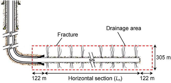
Fig. 1. The typical drainage area of a shale gas well (adapted from reference [38]). |
1.4. Economic evaluation of geological sweet spots
1.4.1. Estimation of shale gas production performance in unevaluated areas
The production performaces of shale gas well differ greatly from conventional gas wells. Shale gas wells exhibit a steep production decline after low long-term production. The production performance of analogous developed shale plays provides an important guidance for estimating the production performance in unevaluated shale plays.
Regarding the analogy study in the previous section, the production performance is estimated based on the technically recoverable reserve of a single well in the study area and the general trend of production performance in the analog play. Fig. 2 shows the estimated 25-year technically recoverable reserve per well in the study area based on the analogous study.
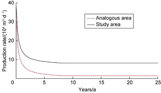
Fig. 2. Technically recoverable reserves per well in the study area, estimated by the analogous study method. |
1.4.2. Drilling plan based on stable production
Sustainable production is one of the factors considered in gas field development, which implies that the production of the sweet spot zone will have a fixed plateau in a period (for example 25 years). Based on the total number of wells in a sweet spot zone and considering the decline rate of single wells during 25 years, the drilling program should be updated so that each sweet spot zone can produce at the maximum allowable production rate. In order to maintain the production plateau, it means that the production decline should be compensated by drilling new wells.
1.4.3. Estimation of economically recoverable reserves of geological sweet spot zones
Economic evaluation contributes to further screening of sweet spot zones. Parameters such as NPV (net present value), IRR (internal rate of return) and payback period can be obtained by using a stochastic method that uses the P10, P50, and P90 values of capital expenditure, discount rate, gas price, and operating expense as the main references.
In this paper, we use the method of Madani et al. [37] to determine the economically recoverable reserves of each sweet spot zone, by defining the geological sweet spot zone with a payback period less than 5 years and IRR higher than 20%.
2. Evaluation of shale gas zones in the Lurestan region
2.1. Geological setting of shale gas in the Lurestan region
Compared with North America, there are less proven shale gas zones in the Middle East. The assessment of unconventional resources resulted in the exploration of two Cretaceous shale gas reservoirs (S1 and S2) in the Lurestan region and the Zagros major reverse fault intersection area in Iran [39⇓⇓⇓-43].
The Lurestan area is located in the Southwest of Iran. It is a part of the Zagros fold-thrust belt, and confined to the Zagros major reverse fault and the Dezful Bay in the northeast and southeast, respectively [44-45]. Both S1 and S2 are mainly composed of shale interlayers with rich organic matter and dark gray micritic limestone[46]. Analysis of shale samples showed that the TOC values of these formations ranged from 1% to 9%[47], and the organic matter type was mainly type II kerogen. Although geological and regional studies have been done, feasibility study and economic evaluation of shale gas development have not so far in this prospect region. The Lurestan area is very large, but no pilot production has been done, so it is urgent to develop a reliable strategy for locating the favorable zones. In this study, we follow the techno-economic workflow to assess the sweet spot zones in the Lurestan area.
2.2. Geological sweet spot zones
A static model of 500 m by 500 m by 5 m was used to screen the geological sweet spot zones in the Lurestan area. The TOC, Ro, H and Gc of every grid of the model are screening parameters. TOC ≥ 2% is the first condition, and then Ro ≥ 1.2%, H ≥ 30 m and Gc ≥ 2.5 m3/t. Eligible cells are shown in green (Fig. 3 a to 3f).
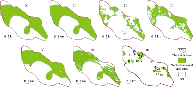
Fig. 3. Schematic representation of shale gas sweet spot zones in the Lurestan area. (a) Zone with Ro ≥ 1.2% in reservoir S1; (b) Zone with Ro ≥ 1.2% in reservoir S2; (c) Zone with Gc ≥ 2.5 m3/t in reservoir S1; (d) Zone with Gc ≥ 2.5 m3/t in reservoir S2; (e) Zone with H ≥ 30 m in reservoir S1; (f) Zone with H ≥ 30 m in reservoir S2; (g) geological sweet spot zones and SN. |
Considering available oil and gas wells, water resources and gas pipelines, we finally selected 21 geological sweet spot zones based on superimposition and ranges of green cells (Fig. 3 g).
2.3. Analogous study of key parameters
The Lurestan shale gas area has not been developed, therefore no production data are available. We determined to get the geological information of the study area through an analogy study from developed shale gas zones. We compared S1 and S2 with Marcellus, Barnett, Woodford, Fayettville, Haynesville, Bossier, Muskwa, Eagle Ford, Utica, and Montney shale gas reservoirs. Table 1 shows the key parameters used for the analogous study, including reservoir depth, fracture density (number of fractures within 30 m), brittle mineral content, adsorbed gas fraction, clay mineral content, pay zone, and pressure gradient.
| Location | Formation | Depth/ m | Fracture density/ (fractures·30 m-1) | Brittle mineral/% | Adsorbed gas/% | Clay mineral/% | H/ m | Pressure gradient/ (MPa·km-1) |
|---|---|---|---|---|---|---|---|---|
| Appalachian Basin, USA | Marcellus | 1905.0 | 10 | 62.0 | 45.0 | 35.0 | 38.10 | 13.78 |
| Mississippian, USA | Barnett | 2286.0 | 9 | 60.0 | 55.0 | 25.0 | 38.10 | 10.85 |
| Oklahoma, USA | Woodford | 2590.8 | 7 | 60.0 | 60.0 | 20.0 | 45.72 | 11.75 |
| Arkansas, USA | Fayettville | 1219.2 | 9 | 47.0 | 60.0 | 38.0 | 41.14 | 9.95 |
| Salt Basin, USA | Haynesville | 3657.6 | 0 | 50.0 | 25.0 | 30.0 | 79.24 | 18.08 |
| Louisiana, USA | Bossier | 3550.9 | 9 | 42.0 | 55.0 | 42.0 | 74.67 | 17.63 |
| Alaska, USA | Muskwa | 2438.4 | 9 | 70.0 | 20.0 | 20.0 | 121.92 | 11.53 |
| Texas, USA | Eagle Ford | 2133.6 | 5 | 75.0 | 25.0 | 15.0 | 60.96 | 11.08 |
| Tunisia | Utica | 1264.9 | 9 | 30.0 | 60.0 | 20.0 | 152.40 | 11.75 |
| Western Canada | Montney | 1920.2 | 10 | 70.0 | 10.0 | 15.0 | 106.68 | 10.17 |
| Lurestan | S1 | 3210.1 | 9 | 88.8 | 34.4 | 6.4 | 75.28 | 10.85 |
| Lurestan | S2 | 3435.1 | 9 | 88.5 | 52.7 | 4.8 | 37.49 | 10.85 |
The least squared differences between the shale reservoir parameters (reservoir depth, fracture density, brittle mineral content, adsorbed gas percentage, clay mineral content, pay zone, and pressure gradient) of the analogous areas and those of S1 and S2 were calculated. The results show that the Eagle Ford shale gas reservoir has the least differences from and the most similar formation conditions to S1 and S2 shale gas reservoirs (Fig. 4 ).
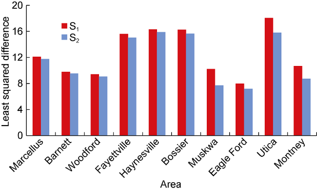
Fig. 4. Comparison of developed shale plates with S1 and S2 formations. |
The recovery and the average length of the horizontal section of Eagle Ford shale gas wells are about 31% and 2029 m, respectively. The probability distribution of this shale gas recovery follows a Pearson type. We extracted the Eagle Ford Shale gas well parameters to set up the development plan and estimate the development cost ion of the S1 and S2 shale gas reservoirs. Fig. 5 shows the Eagle Ford Shale gas production performance, which has been adjusted for the study area.
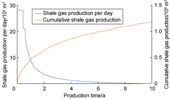
Fig. 5. Eagle Ford single well shale gas production curve (according to reference [49]). |
2.4. Technically recoverable reserves and the number of required wells in each sweet spot zone
It is assumed to have the maximum production plateau for 25 years in each sweet spot zone, which is the base for developing the drilling plan. By inputting geological sweet spot parameters into Eqs. (1)-(4), we got the number of drilling wells, P10, P50, and P90 values of the technically recoverable reserves and the expected ultimate recoverable reserves per well over 25 years (Table 2 ). Both the technically recoverable reserves and the expected ultimate recoverable reserves per well at P10 are higher than those at P50, and P90 in almost all zones. Sweet spot zone No. 1 has the best evaluation, where 458 new wells, i.e. top 2, will be drilled in 25 years, and the technically recoverable reserves at P10, P50, and P90 are 852.2×10⁸, 1058.9×108 and 1364.7×108 m3, respectively, the highest in all zones. The technically recoverable reserves of zones Nos. 1 5, 9, 12, 13, 14, 20, and 21 are not high, and the comprehensive evaluation is poor.
Table 2. Required wells, technically recoverable reserves, and estimated ultimate recoverable reserves per well in every geological sweet spot zone |
| Sweet spot SN | Number of wells per zone | Technically recoverable reserves/108 m3 | Estimated ultimate recoverable reserves per well/104 m3 | ||||
|---|---|---|---|---|---|---|---|
| P90 | P50 | P10 | P90 | P50 | P10 | ||
| 1 | 458 | 852.2 | 1 058.9 | 1 364.7 | 18 633 | 23 107 | 29 818 |
| 2 | 247 | 376.6 | 467.2 | 603.1 | 15 235 | 18 916 | 24 409 |
| 3 | 257 | 348.2 | 430.4 | 557.8 | 13 536 | 16 792 | 21 663 |
| 4 | 130 | 240.7 | 297.3 | 385.1 | 18 491 | 22 937 | 29 591 |
| 5 | 45 | 68.0 | 84.9 | 110.4 | 15 178 | 18 831 | 24 296 |
| 6 | 69 | 135.9 | 169.9 | 220.8 | 19 879 | 24 664 | 31 800 |
| 7 | 241 | 300.1 | 370.9 | 478.5 | 12 431 | 15 404 | 19 879 |
| 8 | 263 | 402.0 | 498.3 | 645.5 | 15 319 | 18 001 | 24 490 |
| 9 | 61 | 70.8 | 87.8 | 113.3 | 11 695 | 14 498 | 18 689 |
| 10 | 175 | 266.1 | 331.3 | 427.5 | 15 263 | 18 916 | 24 409 |
| 11 | 61 | 107.6 | 133.1 | 172.7 | 17 641 | 21 889 | 28 232 |
| 12 | 36 | 48.1 | 59.5 | 76.4 | 13 196 | 16 339 | 21 096 |
| 13 | 32 | 73.6 | 90.6 | 116.1 | 22 795 | 28 289 | 36 501 |
| 14 | 33 | 48.1 | 59.5 | 76.4 | 14 498 | 17 981 | 23 220 |
| 15 | 215 | 235.0 | 291.6 | 373.7 | 10 902 | 13 507 | 17 443 |
| 16 | 520 | 591.7 | 733.3 | 945.6 | 11 383 | 14 102 | 18 208 |
| 17 | 147 | 138.7 | 172.7 | 223.7 | 9 543 | 11 808 | 15 263 |
| 18 | 352 | 410.5 | 509.6 | 659.7 | 11 695 | 14 498 | 18 718 |
| 19 | 81 | 116.1 | 144.4 | 184.1 | 14 272 | 17 698 | 22 824 |
| 20 | 68 | 59.5 | 73.6 | 93.4 | 8 637 | 10 704 | 13 819 |
| 21 | 26 | 28.3 | 36.8 | 45.3 | 11 129 | 13 790 | 17 811 |
2.5. Economic evaluation of geological sweet spot zones
Based on the technically recoverable reserves, the economically recoverable reserves are estimated. Then the number of wells to be drilled is estimated for each sweet spot zone. Assuming to keep the maximum production capacity over 25 years, the number of wells to be drilled in each sweet spot zone is obtained (Table 2 ). Fig. 6 shows the plateau production rate and the number of wells in each sweet spot zone.
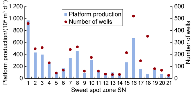
Fig. 6. Number of wells and platform production in the sweet spot zones. |
A cash flow model was constructed based on the premise that gas wells will produce over 25 years. The model is based on a stochastic approach that accounts for gas recovery and economic parameters (gas price, discount rate, drilling & completion costs, and operating cost), P10, P50 and P90, and well production capacity. Without any experience in developing shale gas in Iran, we selected geological sweet spot zones and carried out economical evaluation by referring to the development costs of the Eagle Ford shale gas. Fig. 7 shows the capital expenditures of Eagle Ford shale gas, of which drilling and completion costs account for up to 80%. Drilling costs are related to rig rental, drilling fluid, casing, cement, and so on, accounting for 32%. Completion costs mainly cover fracturing pumps, fracturing equipment, proppants, completion fluids, and flowback fluids, accounting for 48%. Expenses other than well drilling and completion are mainly for artificial lift, equipment, insurance, and technical consulting, accounting for approximately 20%.
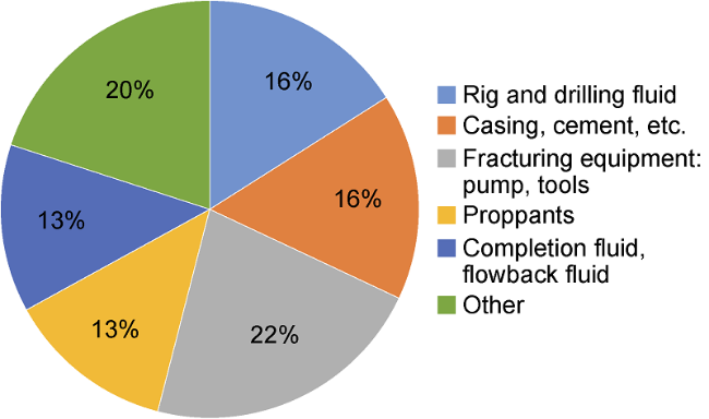
Fig. 7. Capital expenditure breakdown and share of Eagle Ford shale gas. |
The unit development cost of Eagle Ford shale gas depends on many factors [6]. This study uses a probability distribution to analyze the economics of shale gas wells in S1 and S2 reservoirs, rather than referring to the exact values of drilling and completion costs (Table 3 ). Remaining costs are estimated based on their weights.
Table 3. Shale gas recovery and economic parameters in the Lurestan area |
| Completion cost per section/106 $ | Drilling cost/($·m-1) | Operating cost/(10-3 $·m-3) | |||||||||||||||
|---|---|---|---|---|---|---|---|---|---|---|---|---|---|---|---|---|---|
| Distribution Map | Normal distribution value | P10 | P50 | P90 | Distribution Map | Normal distribution value | P10 | P50 | P90 | Distribution Map | Normal distribution value | P10 | P50 | P90 | |||
| Standard | 0.19 | 0.18 | 0.19 | 0.20 | Standard | 426.53 | 393.72 | 426.53 | 459.34 | Standard | 48.74 | 42.74 | 48.74 | 54.39 | |||
| Natural gas prices/(10-3 $·m-3) | Discount rate/% | Recovery/% | |||||||||||||||
| Distribution Map | Normal distribution value | P10 | P50 | P90 | Distribution Map | Normal distribution value | P10 | P50 | P90 | Distribution Map | Normal distribution value | P10 | P50 | P90 | |||
| Triangular | 149.05 | 199.91 | 123.62 | 105.96 | Standard | 15 | 12 | 15 | 18 | Pearson type | 32.16 | 40.00 | 31.00 | 25.00 | |||
The drilling and completion costs per well are estimated by assuming that the well is two-branch. Fig. 8 shows the schematic map of a completed well in the S1 and S2 formations, where the green boxes means the fracturing locations and the numbers of fracturing stages. The horizontal section length, unit drilling cost, the number of fracturing stages in the horizontal section, and unit completion cost are estimated based on the data of Eagle Ford shale gas.
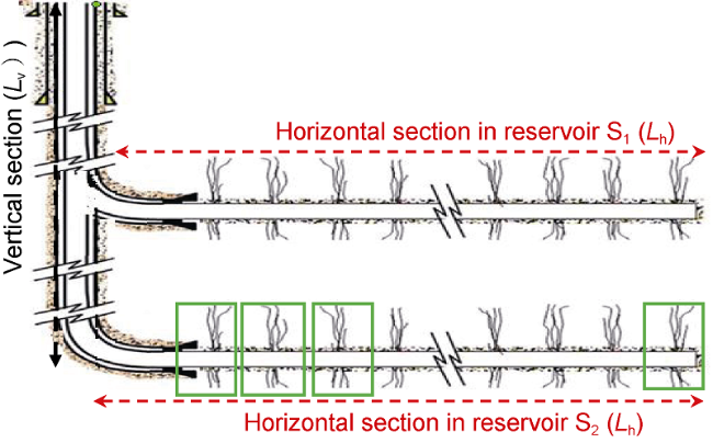
Fig. 8. Schematic diagram of shale gas drilling and completion in the Lurestan area. |
Cd=(Lv+2Lh)Cdu
Cc=2nCcu
Table 4. Basic data of geological sweet spot zones in the Lurestan area |
| SN | Area/km2 | Geological gas reserves in S1/108 m3 | Geological gas reserves in S2/108 m3 | S1 depth/m | S2 depth/m |
|---|---|---|---|---|---|
| 1 | 317 | 2370 | 1 070 | 2865 | 3066 |
| 2 | 171 | 1506 | 558 | 3037 | 3184 |
| 3 | 178 | 1393 | 541 | 2822 | 2967 |
| 4 | 90 | 963 | 419 | 3701 | 3944 |
| 5 | 31 | 275 | 127 | 3281 | 3481 |
| 6 | 48 | 549 | 249 | 3728 | 3904 |
| 7 | 167 | 1198 | 513 | 2828 | 2992 |
| 8 | 182 | 1611 | 714 | 2376 | 2542 |
| 9 | 42 | 286 | 139 | 2223 | 2404 |
| 10 | 121 | 1068 | 464 | 2783 | 2970 |
| 11 | 42 | 430 | 167 | 3912 | 4184 |
| 12 | 25 | 190 | 85 | 4017 | 4258 |
| 13 | 22 | 292 | 127 | 4031 | 4342 |
| 14 | 23 | 193 | 76 | 3219 | 3531 |
| 15 | 149 | 937 | 368 | 3021 | 3218 |
| 16 | 360 | 2367 | 926 | 4180 | 4518 |
| 17 | 102 | 561 | 255 | 3071 | 3351 |
| 18 | 244 | 1648 | 685 | 3613 | 3860 |
| 19 | 56 | 462 | 178 | 3189 | 3476 |
| 20 | 47 | 235 | 105 | 3357 | 3554 |
| 21 | 18 | 116 | 48 | 2161 | 2391 |
The operating cost of Eagle Ford shale gas ranges from 45.9 to 97.5 $/103 m3, including water treatment, disposal, equipment maintenance, wellhead equipment, pump fuel, and general overhead (mainly labor costs). Considering the different categories of costs and their weights in Eagle Ford shale gas development, this study delineates an appropriate operating cost range by making appropriate adjustments.
Commercial shale gas production depends critically on wellhead gas price and is considered as an external uncertainty, affected by many factors. In our study, the lowest gas price is the bottom gas price in the petrochemical industry of Iran, while the highest gas price is the export gas price to neighboring countries. Table 3 lists the highest and lowest gas prices and their distribution.
Regarding the aforementioned costs and prices, the estimated NPVs at P90 and P50 are negative for all sweet spot zones. They aren’t economical (Fig. 9 ).
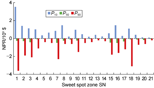
Fig. 9. NPV of geological shale gas sweet spot zones in the Lurestan area at P10, P50 and P90. |
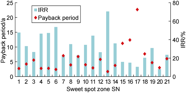
Under an optimistic condition (NPV at P10), the NPVs of all geological sweet spot zones are positive. But their economically recoverable reserves should be further estimated. Fig. 10 shows the IRR and payback period of the geological sweet spot zones in the Lurestan region. When IRR is higher than 20% and the maximum payback is less than 5 years, 11 geological sweet spot zones are commercial to develop, which are Nos. 1, 2, 4, 5, 6, 8, 10, 11, 13, 14 and 19. The total technically recoverable reserves are 7875×108 m3 and economically recoverable reserves are 4306×108 m3. Of them, No. 1 has the highest value of commercial development, the highest NPR of 35×108 $, and the highest plateau rate over 25 years.
Fig. 10. IRR and payback period of the geological shale gas sweet spot zones in the Lurestan area (based on the development costs of Eagle Ford shale gas). |
3. Conclusions
A multi-parameter evaluation method that takes economic and technical indicators into account is proposed for selecting the technical and economic sweet spot zones in unevaluated shale gas plays. The method includes four steps: (1) identification of geological sweet spot zones; (2) analogy study of key parameters; (3) estimation of technically recoverable reserves and the number of wells required to completely cover the sweet spot zones; and (4) economical evaluation of geologi sweet spots. Key parameters include H, TOC, Ro and Gc.
An analogy study was conducted on the Cretaceous shale gas in the Lurestan area by referring to the development of Eagle Ford shale gas. The results show that the key parameters of the Eagle Ford shale gas formations are comparable with the S1 and S2 formations in the Lurestan area. The commercial development value is not high in terms of NPV at P50 and P90, but at P10, the total technically recoverable reserves and economically recoverable reserves of 21 geological sweet spot zones are 7875×108 m3 and 4306×108 m3, respectively, and of which 11 sweet spot zones are expected to be commercial, especially the No. 1 sweet spot zone that has the highest commercial development value with NPV of 35×108 $.
Nomenclature
Ags—area of a sweet spot, m2;
Cc—completion cost, $;
Ccu—completion cost per section, $/section;
Cd—drilling cost, $;
Cdu—drilling cost per meter, $/m;
Er—recovery, %;
EUR—expected ultimate recovery, 108 m3;
G—original geological reserve of single sweet spot, 108 m3;
Gc—gas per ton, m3/t;
Ge—economically recoverable reserves, 108 m3;
Gt—technically recoverable reserves, 108 m3;
H—pay zone, m;
Lh—length of horizontal section, m;
Lv—length of vertical section, m;
n—number of fractured stages in a horizontal section;
Nw—number of wells;
P10—cumulative probability of 10 %;
P50—cumulative probability of 50 %;
P90—cumulative probability of 90 %;
Ro—vitrinite reflectance, %;
Sw—drainage area, m2;
TOC—total organic carbon content, %.