

Introduction
Shale oil is generally stored in organic-rich shale with permeability of less than 0.1×10⁻³ μm2 and porosity of less than 10% [1-2]. One of the main methods to improve shale oil recovery is to greatly increase the drainage area by adopting long horizontal wells and multi-stage and multi-cluster volume fracturing. Field production data indicate that even with the adoption of volume fracturing and long horizontal well, a large number of shale wells are still not commercially viable [3]. Fracturing-soaking technology provides a new idea for shale oil development[4]. The Changqing, Qinghai, Daqing, Jilin and other oil fields have adopted the production management system of "fracturing, soaking and re-production" in some shale oil blocks successively, and achieved good stimulation effect. At present, most shale oil wells in China are shut in for 14-60 d after fracturing, and the determination of shut-in time mostly, without scientific and reasonable basis, depends largely on the experience of operators [5-6]. Establishing the optimization model and method of shut-in time after fracturing is the key to the implementation of the fracturing and soaking, and the theoretical and engineering issue needs to be solved for further improving shale oil recovery.
The purpose of fracturing is to reconstruct the reservoir to obtain larger fracture distribution area and increase the high-permeability volume space for oil and gas flow. The purpose of shut-in is to increase the flow energy of formation fluid and enhance the imbibition effect of oil-water displacement by utilizing a large amount of fracturing fluid retained in the reservoir based on the coupling effect of fluid flow, imbibition principle and chemical reaction, and finally achieve the purpose of increasing crude oil production [7]. Although simple in operation, shut-in is very complex in core physical mechanism. Lee et al. [8⇓⇓⇓⇓-13] mainly studied the imbibition behavior dominated by gravity and capillary pressure at the core scale and field scale by lab experiment and numerical simulation. They concluded that the change of rock wettability and complexity of reservoir reconstruction were important factors affecting the stimulation effect of soaking. Li et al. [14⇓⇓⇓⇓-19] considered the laminar flow caused by chemical potential and the influence of osmotic pressure besides the capillary pressure dominated imbibition on the stimulation effect of soaking. They found that the difference of salinity inside and outside the matrix in the process of soaking was the fundamental reason for generating osmotic pressure and promoting crude oil displacement. Bui et al. [20-22] also mentioned in their study that the elastic energy of the reservoir would be supplemented due to the filtration of fracturing fluid into the reservoir, which might also lead to the increase of productivity after shut-in. If the reservoir is deemed oil wet, adding surfactant to the fracturing fluid can further improve the wettability of the reservoir through the fluid flow during shut-in to increase production. Generally speaking, most of the researchers studied the mechanisms of imbibition oil recovery during shut-in, and rarely examined the optimal shut-in time after fracturing. Although carrying out a detailed study on the optimal soaking time, Wang et al.[23] didn’t consider the influence of osmotic pressure on imbibition in the model and the multiphase flow in hydraulic fractures, and the physical model they established wasn’t a complete filed scale model.
This work aims to establish an integrated shut-in time optimization model of fracturing, soaking and production for shale oil reservoir, and puts forward a soaking time optimization method with the goal of maximizing productivity considering the effects of capillary pressure, chemical potential, osmotic pressure and hydraulic fractures. The model has been verified by an application example and commercial software. In the integrated simulation process of fracturing-soaking-production, the key production-increasing mechanism of soaking has been analyzed from multiple angles, and the influence laws of different factors on the optimal soaking time of shale oil development have been investigated emphatically, so as to guide the decision-making of soaking time after fracturing of shale oil horizontal wells and provide a theoretical basis for further optimization of shut-in system.
1. Optimization model for shut-in time in fracturing-soaking-production
1.1. Assumptions and physical model
Assumptions: (1) The model includes three continuous physical processes of fracturing, soaking and production. Fracturing is an injection process with large injection rate in a short time under the condition of constant hydraulic fracture length; soaking is a process of self-equilibrium imbibition in shale oil reservoir with the end of fracturing as the initial condition and the source sink term as zero; production is a recovery process with the end of shut-in as the initial condition. (2) The physical model is a multi-segment and multi-cluster model of horizontal well. The imbibition and multiphase flow between oil and water mainly occur between hydraulic fractures and matrix. (3) There is three-phase isothermal flow of oil, water and solute in the reservoir. (4) The compressibility of cracks and matrix is considered, and the solute is an incompressible phase. (5) The effects of matrix capillary pressure, osmotic pressure, membrane effect and elastic properties are considered.
According to the above assumptions, the optimization model of multi-stage and multi-cluster fracturing-soaking-production integrated shut-in time of shale oil horizontal well has been established as shown in Fig. 1 . In the model, the horizontal well is along the x-axis direction, and the hydraulic fracture is perpendicular to the horizontal well and parallel to the y-axis. The fracture section length, cluster number and fracture length are obtained by fitting the field fracturing pressure data. During fracturing, fracturing fluid is injected into hydraulic fractures through the wellbore under high pressure, and then filtered into the reservoir. The amount of filtration is expressed by the flow exchange term between matrix and hydraulic fracture. After fracturing, the source term is zero. At this time, the fracturing fluid in hydraulic fractures will continue to flow into the matrix under the action of differential pressure, and the oil phase in the matrix will enter the hydraulic fractures under the action of capillary pressure, chemical potential and osmotic pressure. Based on the physical state after shut-in, the oil and water production at different soaking moments can be obtained through productivity simulation. Productivity simulation is carried out based on the physical property state at the end of soaking, finally the soaking time after fracturing with the goal of maximizing productivity can be obtained from the simulation.
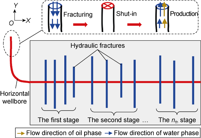
Fig. 1. Fracturing-soaking-production integrated soaking time optimization model. |
1.2. Mathematical model
1.2.1. Continuity equation of oil and water in matrix and fracture
It is assumed that the solute is an incompressible phase and only soluble in the water phase. Based on the law of mass conservation, Darcy's law and Van’t Hoff's law, considering the influence of capillary pressure and osmotic pressure in static spontaneous infiltration, the continuity equation of oil and water phase in matrix unit can be expressed as [24⇓-26]:
$\nabla \cdot \left[ {{K}_{\text{m}}}{{\lambda }_{\text{wm}}}\nabla \left( {{p}_{\text{wm}}}-{{\gamma }_{\text{w}}}{{D}_{\text{m}}} \right)-{{\lambda }_{\text{wm}}}\frac{{{K}_{\text{m}}}}{{{V}_{\text{w}}}}\omega R{{T}_{\text{m}}}\nabla {{c}_{\text{sm}}} \right]- \\ {{q}_{\text{wmf}}}=\frac{\partial }{\partial t}\left[ \left( 1-{{\varepsilon }_{\text{vm}}} \right){{S}_{\text{wm}}}{{\phi }_{\text{m}}} \right]$
$\nabla \cdot \left[ {{K}_{\text{m}}}{{\lambda }_{\text{om}}}\nabla \left( {{p}_{\text{om}}}-{{\gamma }_{\text{o}}}{{D}_{\text{m}}} \right) \right]-{{q}_{\text{omf}}}= \frac{\partial }{\partial t}\left[ \left( 1-{{\varepsilon }_{\text{vm}}} \right){{S}_{\text{om}}}{{\phi }_{\text{m}}} \right]$
The first term on the left of Eq. (1) is the water phase flow term, which is composed of Darcy laminar flow term of water and water phase diffusion term caused by solute concentration difference in matrix pores. The second term represents the water phase exchange term between matrix and fracture. Hydraulic fractures are characterized by embedded discrete model, and the mass transfer relationship between matrix and fracture is established by introducing the conductivity coefficient (Tomf and Twmf) between matrix and fracture. Considering the influence of membrane effect and osmotic pressure on water phase flow, but not on oil phase flow, the osmotic pressure difference $\Delta {{p}_{\text{op}}}=\frac{\omega R{{T}_{\text{m}}}}{{{V}_{\text{w}}}}\Delta {{c}_{\text{smf}}}$ is substituted into the exchange term, then the exchange term can be expressed as [24]:
${{q}_{\text{wmf}}}=\frac{{{\lambda }_{\text{wmf}}}{{T}_{\text{wmf}}}}{{{V}_{\text{m}}}}\left( \Delta {{p}_{\text{wmf}}}+\Delta {{p}_{\text{op}}} \right)=\frac{{{\lambda }_{\text{wmf}}}{{T}_{\text{wmf}}}\Delta {{p}_{\text{wmf}}}}{{{V}_{\text{m}}}}+\frac{{{\lambda }_{\text{wmf}}}{{T}_{\text{wmf}}}}{{{V}_{\text{m}}}}\frac{\omega R{{T}_{\text{m}}}}{{{V}_{\text{w}}}}\Delta {{c}_{\text{smf}}}$
${{q}_{\text{omf}}}=\frac{{{\lambda }_{\text{omf}}}{{T}_{\text{omf}}}\Delta {{p}_{\text{omf}}}}{{{V}_{\text{m}}}}$
The first term on the right side of Eq. (3) represents the flow term driven by pressure gradient, and the second term represents the flow term driven by osmotic pressure between matrix and fracture.
Due to high conductivity of fracture, hydraulic diffusion in fracture is fast, so compared with the effect of solute concentration diffusion on water phase flow in matrix, the solute concentration diffusion in the fracture has less influence on the water phase flow. Therefore, the influences of solute and capillary pressure are ignored. Based on Eqs. (1)-(4), one-dimensional flow equations of oil and water in hydraulic fractures can be deduced:
$\nabla \cdot \left[ {{K}_{\text{f}}}{{\lambda }_{\text{wf}}}\nabla \left( {{p}_{\text{wf}}}-{{\gamma }_{\text{w}}}{{D}_{\text{m}}} \right) \right]+{{q}_{\text{wmf}}}+{{q}_{\text{wf}}}\text{=}\frac{\partial }{\partial t}\left( {{\phi }_{\text{f}}}{{S}_{\text{wf}}} \right)$
$\nabla \cdot \left[ {{K}_{\text{f}}}{{\lambda }_{\text{of}}}\nabla \left( {{p}_{\text{of}}}-{{\gamma }_{\text{o}}}{{D}_{\text{m}}} \right) \right]+{{q}_{\text{omf}}}+{{q}_{\text{of}}}\text{=}\frac{\partial }{\partial t}\left( {{\phi }_{\text{f}}}{{S}_{\text{of}}} \right)$
In the process of injection, the source item adopts constant flow injection. In the production process, the sink term takes the oil production at fixed bottomhole pressure. In this case, the well index calculated for productivity can refer to the equivalent well index within fracture element derived by Moinfar et al. [25-26] based on the Peaceman well model.
1.2.2. Continuity equation of chemical solute in matrix and fracture
Based on the law of mass conservation and van't Hoff's law, considering the solute diffusion caused by Darcy flow of water phase in matrix, the solute laminar flow caused by concentration difference of solute and the influence of osmotic pressure inside and outside matrix, the solute continuity equation in matrix element can be derived [24,27]:
$\nabla \cdot \left\{ {{c}_{\text{sm}}}{{K}_{\text{m}}}{{\lambda }_{\text{wm}}}\left( \omega +\frac{{{\rho }_{\text{w}}}}{{{\rho }_{\text{s}}}}\frac{{{c}_{\text{sm}}}}{1-{{c}_{\text{sm}}}} \right)\left[ \nabla \left( {{p}_{\text{wm}}}-{{\gamma }_{\text{w}}}{{D}_{\text{m}}} \right)- \right. \right. \\ \left. \left. \frac{\omega R{{T}_{\text{m}}}}{{{V}_{\text{w}}}}\nabla {{c}_{\text{sm}}} \right]+{{\phi }_{\text{m}}}{{D}_{\text{eff}}}\nabla {{c}_{\text{sm}}} \right\}-{{q}_{\text{smf}}}= \\ \frac{\partial }{\partial t}\left[ \left( 1-{{\varepsilon }_{\text{vm}}} \right)\frac{{{\rho }_{\text{w}}}}{{{\rho }_{\text{s}}}}{{S}_{\text{wm}}}{{\phi }_{\text{m}}}\frac{{{c}_{\text{sm}}}}{1-{{c}_{\text{sm}}}} \right] $
Since the surface of the rock block is not a perfect permeable membrane, some ions can also pass through when water molecules are allowed to pass through (the ability of ions to pass through depends on the membrane coefficient). The solute exchange term between fracture and matrix can be expressed as:
${{q}_{\text{smf}}}\text{=}\frac{{{c}_{\text{swmf}}}}{1-{{c}_{\text{swmf}}}}\frac{{{\rho }_{w}}}{{{\rho }_{\text{s}}}}{{q}_{\text{wmf}}}$
Substituting Eq. (3) into Eq. (8), the following equation can be obtained:
${{q}_{\text{smf}}}\text{=}\frac{{{c}_{\text{swmf}}}}{1-{{c}_{\text{swmf}}}}\frac{{{\rho }_{w}}}{{{\rho }_{\text{s}}}}\left( \frac{{{\lambda }_{\text{wmf}}}{{T}_{\text{wmf}}}\Delta {{p}_{\text{wmf}}}}{{{V}_{\text{m}}}}+ \\ \right. \left. \frac{{{\lambda }_{\text{wmf}}}{{T}_{\text{wmf}}}}{{{V}_{\text{m}}}}\frac{\omega R{{T}_{\text{m}}}}{{{V}_{\text{w}}}}\Delta {{c}_{\text{smf}}} \right)$
As for solute flow in fractures, although solute flow has little influence on oil-water flow, the fast oil-water flow velocity has great influence on solute distribution due to the influence of high conductivity of fractures. Therefore, the influence of oil-water flow on solute flow in fracture should be considered. Without considering the influence of solute diffusion in the fracture and assuming that solute isn’t soluble in the oil phase, the continuity equation of solute transport in the fracture can be obtained:
$\nabla \cdot \left[ {{c}_{\text{sf}}}{{K}_{\text{f}}}{{\lambda }_{\text{wf}}}\nabla \left( {{p}_{\text{wf}}}-{{\gamma }_{\text{w}}}{{D}_{\text{m}}} \right) \right]+\frac{{{\rho }_{\text{s}}}}{{{\rho }_{\text{w}}}}{{q}_{\text{smf}}}+ \\ \frac{{{c}_{\text{sf,in,pro}}}}{1-{{c}_{\text{sf,in,pro}}}}{{q}_{\text{wf}}}=\frac{\partial }{\partial t}\left( {{S}_{\text{wf}}}{{\phi }_{\text{f}}}{{c}_{\text{sf}}} \right)$
1.2.3. Auxiliary equation
To solve the six nonlinear equations of oil-water flow continuity and solute continuity, a series of auxiliary equations are needed. The formation is elastic, so the compressibility of fractures and matrix needs to be considered. Then the stress-sensitive equations of porosity and permeability can be expressed as:
$\left\{ \begin{align} & {{\phi }_{\text{m}}}={{\phi }_{0,m}}{{\text{e}}^{{{C}_{\text{m}}}\left( {{p}_{\text{om}}}-{{p}_{0}} \right)}} \\ & {{\phi }_{\text{f}}}={{\phi }_{0,\text{f}}}{{\text{e}}^{{{C}_{_{\text{f}}}}\left( {{p}_{{{\text{o}}_{\text{f}}}}}-{{p}_{0}} \right)}} \\ \end{align} \right.$
$\left\{ \begin{align} & {{K}_{\text{m}}}={{K}_{0,m}}{{\text{e}}^{{{E}_{\text{m}}}\left( {{p}_{\text{om}}}-{{p}_{0}} \right)}} \\ & {{K}_{\text{f}}}={{K}_{0,\text{f}}}{{\text{e}}^{{{E}_{_{\text{f}}}}\left( {{p}_{{{\text{o}}_{\text{f}}}}}-{{p}_{0}} \right)}} \\ \end{align} \right.$
The saturation equations are:
$\left\{ \begin{align} & {{S}_{\text{om}}}+{{S}_{\text{wm}}}=1 \\ & {{S}_{\text{of}}}+{{S}_{\text{wf}}}=1 \\ \end{align} \right. $
For the water-wet reservoir rock, the water phase is the wetting phase, and the oil phase is the non-wetting phase, so the capillary pressure equation is:
${{p}_{\text{c}}}\left( {{S}_{\text{wm}}} \right)={{p}_{\text{om}}}-{{p}_{\text{wm}}}$
1.2.4. Initial condition and boundary condition
In the simulation, fracturing, soaking and production are three continuous physical processes. The reservoir parameters at the end of fracturing are the initial parameters of soaking, and the reservoir parameters at the end of soaking are the initial parameters of production simulation. Thus, by setting the initial reservoir parameters during fracturing, the production dynamics after a certain soaking time can be simulated by the integrated model. In this study, the reservoir is assumed homogeneous, two-dimensional and closed; the matrix and hydraulic fracture before fracturing are assumed same in initial fluid pressure, initial water saturation, initial porosity and initial permeability, and these parameters are obtained from log data of a shale oil well. The length and conductivity of hydraulic fractures are obtained by the inversion of pressure curve during fracturing operation.
1.3. Model calculation
With the calculation accuracy guaranteed and calculation cost controlled, the finite difference method was used to discretize Eqs. (1), (2), (5), (6), (7) and (10), combined with auxiliary equations, initial conditions and boundary conditions, the implicit method was used to solve the pressure and saturation, and the explicit method was used to solve the solute concentration distribution. Based on the discrete forms of Eqs. (1), (2), (5) and (6), the implicit solution matrices of oil phase and water phase were obtained [28]. Similarly, the matrices of Eqs. (7) and (10) were obtained by sorting and simplifying the discrete forms of them. Combining the above two matrix equations, a discrete large sparse matrix system was obtained. This matrix was solved by using computing statement in MATLAB.
1.4. Model validation
Two shale oil wells A and B in Lucaogou Formation shale oil reservoir of Jimusar depression, Junggar Basin were taken as examples to validate the model. These two wells had the same target reservoir, so it was assumed that the target reservoirs were same in physical properties and homogeneous. In addition, it was assumed that the fracture conductivity was uniformly distributed, and the equivalent fracture conductivity was used to replace the non-uniformly distributed conductivity. The reservoir rock had an elastic modulus of 38 GPa, a Poisson's ratio of 0.2, and a fracture toughness of 2 MPa·m1/2. The fracturing parameters of the two wells are shown in Table 1 , with the same type of fracturing fluid. Well A was shut in for 37 d after fracturing, and then opened for production; Well B was directly opened for production after fracturing. Firstly, according to the logging data and field fracturing pressure data, the net pressure was fitted by commercial software to obtain fracture parameters of the two wells after fracturing (Table 2 ), and then the microseismic monitoring data of the two wells (Table 3 and Fig. 2 ) were used for correction. Considering that the fitting data were high in reliability and the microseismic data were overestimated, the principle of correction was to take the smaller one in them. The corrected fracture parameters were arithmetically averaged to get the final basic parameters: for Well A with a total length of the horizontal section of 1200 m, well spacing of 450 m, 15 stages fractured, and an average of 4 clusters of hydraulic fractures in each stage, the fractures had an average half-length of 135 m and average conductivity of 70 × 10-3 μm2·m; for Well B with a total length of the horizontal section of 1200 m, a well spacing of 400 m, 12 fractured stages, and an average of 4 clusters of hydraulic fractures in each stage, the fractures had an average half-length of 140 m and an average conductivity of 80 × 10-3 μm2·m. In addition, the oil-water relative permeability curve and capillary pressure curve of the two wells were the same set of data in the simulation, and were measured from core experiments in lab, as shown in Fig. 3 . Other major input parameters are shown in Table 4 .
Table 1. Main fracturing parameters of Well A and Well B |
| Well name | Stage No. | Stage length/m | Number of perforation clusters | Perforation density/ (number•m-1) | Injection rate/ (m3•min-1) | Total liquid volume/ m3 | Volume of proppant/m3 |
|---|---|---|---|---|---|---|---|
| A | A01 | 80 | 5 | 10 | 8 | 1 000 | 57.6 |
| A02 | 72 | 5 | 12 | 9 | 1 000 | 56.0 | |
| A03 | 90 | 4 | 10 | 10 | 1 200 | 55.3 | |
| A04 | 85 | 5 | 10 | 10 | 1 300 | 60.0 | |
| A05 | 74 | 5 | 10 | 12 | 1 400 | 76.8 | |
| A06 | 78 | 4 | 12 | 14 | 1 400 | 76.6 | |
| A07 | 90 | 4 | 12 | 16 | 1 600 | 92.8 | |
| A08 | 70 | 3 | 12 | 16 | 1 600 | 96.0 | |
| A09 | 80 | 4 | 10 | 15 | 1 600 | 88.4 | |
| A10 | 75 | 4 | 12 | 15 | 1 400 | 80.6 | |
| A11 | 75 | 4 | 12 | 16 | 1 500 | 86.4 | |
| A12 | 80 | 5 | 10 | 16 | 1 500 | 92.0 | |
| A13 | 84 | 4 | 10 | 16 | 1 600 | 92.8 | |
| A14 | 86 | 5 | 10 | 16 | 1 750 | 102.4 | |
| A15 | 82 | 5 | 12 | 16 | 1 600 | 97.6 | |
| B | B01 | 80 | 5 | 10 | 9 | 900 | 53.8 |
| B02 | 90 | 4 | 10 | 10 | 1 000 | 60.4 | |
| B03 | 70 | 4 | 12 | 10 | 1 200 | 64.0 | |
| B04 | 85 | 4 | 12 | 12 | 1 350 | 70.0 | |
| B05 | 85 | 5 | 12 | 13 | 1 450 | 76.0 | |
| B06 | 95 | 5 | 10 | 13 | 1 500 | 86.4 | |
| B07 | 90 | 5 | 10 | 14 | 1 700 | 106.7 | |
| B08 | 80 | 4 | 12 | 14 | 1 600 | 98.4 | |
| B09 | 75 | 4 | 10 | 16 | 1 600 | 96.6 | |
| B10 | 75 | 4 | 10 | 16 | 1 500 | 92.0 | |
| B11 | 80 | 5 | 10 | 16 | 1 500 | 89.2 | |
| B12 | 80 | 5 | 12 | 15 | 1 600 | 105.0 |
Table 2. Fracture parameters obtained from net pressure fitting |
| Well name | Stage No. | Opened fracture/ cluster | Single-stage equivalent fracture Half-length/m | Single-stage equivalent conductivity/(10-3 μm2·m) |
|---|---|---|---|---|
| A | A01 | 3 | 100 | 53.6 |
| A02 | 4 | 120 | 63.5 | |
| A03 | 4 | 126 | 66.3 | |
| A04 | 4 | 127 | 68.8 | |
| A05 | 4 | 140 | 70.5 | |
| A06 | 3 | 153 | 73.5 | |
| A07 | 4 | 134 | 78.0 | |
| A08 | 3 | 145 | 72.2 | |
| A09 | 4 | 148 | 68.5 | |
| A10 | 4 | 158 | 72.1 | |
| A11 | 4 | 126 | 69.5 | |
| A12 | 4 | 121 | 69.0 | |
| A13 | 3 | 160 | 72.4 | |
| A14 | 5 | 141 | 78.0 | |
| A15 | 4 | 138 | 68.5 | |
| B | B01 | 3 | 94 | 58.0 |
| B02 | 3 | 123 | 72.3 | |
| B03 | 4 | 136 | 75.8 | |
| B04 | 4 | 138 | 80.6 | |
| B05 | 4 | 135 | 78.5 | |
| B06 | 4 | 151 | 86.5 | |
| B07 | 5 | 152 | 85.6 | |
| B08 | 3 | 160 | 86.9 | |
| B09 | 3 | 164 | 86.5 | |
| B10 | 4 | 152 | 88.6 | |
| B11 | 4 | 138 | 75.3 | |
| B12 | 5 | 136 | 89.3 |
Table 3. Microseismic monitoring of fracture length and orientation |
| Well name | Stage No. | Mean fracture half-length/m | Orientation/ (°) |
|---|---|---|---|
| A | A01 | 105 | 90/300 |
| A02 | 125 | 280/60 | |
| A03 | 126 | 280/90 | |
| A04 | 130 | 100/270 | |
| A05 | 132 | 80/280 | |
| A06 | 160 | 90/285 | |
| A07 | 146 | 80/270 | |
| A08 | 155 | 110/300 | |
| A09 | 150 | 70/250 | |
| A10 | 155 | 60/260 | |
| A11 | 130 | 260/70 | |
| A12 | 125 | 80/250 | |
| A13 | 165 | 100/250 | |
| A14 | 145 | 100/280 | |
| A15 | 140 | 90/290 | |
| B | B01 | 100 | 100/270 |
| B02 | 133 | 270/80 | |
| B03 | 145 | 260/90 | |
| B04 | 135 | 90/280 | |
| B05 | 140 | 70/280 | |
| B06 | 165 | 80/280 | |
| B07 | 155 | 90/300 | |
| B08 | 165 | 95/280 | |
| B09 | 170 | 80/260 | |
| B10 | 163 | 80/270 | |
| B11 | 146 | 270/80 | |
| B12 | 142 | 90/255 |
Table 4. Main input parameters in model validation |
| Parameter | Value | Parameter | Value |
|---|---|---|---|
| Initial pore pressure | 33.5 MPa | Matrix porosity | 8% |
| Initial water saturation | 40% | Matrix permeability | 0.02×10⁻³ μm2 |
| Initial salinity of formation water | 60 000×10-6 | Membrane efficiency | 6% |
| Initial salinity of fracturing fluid | 1000×10-6 | Effective volume diffusion coefficient | 0.36×10⁻⁹ m2/s |
| Oil phase viscosity | 10 mPa∙s | Water phsae viscosity | 2 mPa∙s |
| Bottom hole pressure | 20 MPa | Gas constant | 8.314 J/(mol∙K) |
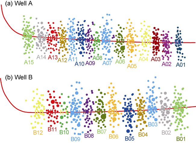
Fig. 2. Micro-seismic monitoring cloud image. |
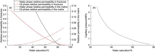
Fig. 3. Oil-water relative permeability (a) and capillary pressure (b) curves. |
Based on the basic parameters of these two wells, the model in this paper was used for physical modeling and simulation. The simulation results are in good agreement with the production data of field statistics (Fig. 4 ), and the simulation results of Well B by Eclipse software also match the simulation results of the model in this paper, proving that this model can accurately predict the production performance with or without soaking.
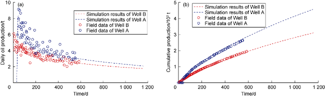
Fig. 4. Comparison between simulation results and production data from field statistics. |
2. Optimization method of shut-in time
Imbibition production is an important mechanism for enhancing oil recovery of shale oil reservoir. Besides capillary pressure and gravity, chemical osmotic pressure, membrane properties of matrix wall and fluid exchange area between matrix and fracture are also important factors affecting imbibition during shut-in. Regardless of fluid damage, at different shut-in times, the displaced oil amount by imbibition and cumulative production are different. With the increase of shut-in time, the cumulative production or recovery increase to a certain extent.
Based on the established fracturing-soaking-production integrated model, a shut-in time optimization method aiming at maximizing productivity and recovering cost fastest has been proposed in this paper. The specific operation steps are as follows.
(1) According to the established model, the recovery performance under a certain set of engineering parameters, geological parameters and a certain shut-in time is obtained.
(2) Change the shut-in time and repeat step (1). Under the same geological parameters and engineering parameters, the relationship between cumulative output and production time under different shut-in time can be obtained, as shown in Fig. 5 a.
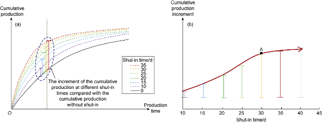
Fig. 5. Schematic diagram of shut-in time optimization method. |
(3) Based on the results of step (2), sort out the differences in cumulative production between different shut-in time schemes and non-soaking scheme at a certain production time (generally select the time point with large difference in cumulative productions), so as to obtain the relationship between the cumulative production increment and shut-in time shown in Fig. 5 b.
(4) Based on Fig. 5 b, the optimal shut-in time is picked out. In order to select the optimal shut-in time quantitatively and ensure that the cumulative production increment basically reaches the peak value within the shortest shut-in time, the first derivative of the relation curve between the cumulative production increment and shut-in time can be calculated. When its value is 0.001 t/d, that is, the slope of a point on the curve is 0.001 t/d, the corresponding shut-in time of this point is considered as the optimal shut-in time. As shown in Fig. 5 b, the slope at point A is 0.001 t/d, and the corresponding optimal shut-in time is 30 d. At this point, the flow of oil, water and solute in the system is basically in equilibrium state, and the cumulative production increment is reaching the peak. If the well remains shut-in for longer, the increase of cumulative production increment is small. The shut-in time of 30 d can achieve the goal of the fastest cost recovery.
3. Case study
The optimal shut-in time is the time for the multi- phase fluid flow and energy distribution to re-balance again in reservoir after fracturing and is a key design parameter in the soaking decision. According to the integrated fracturing-soaking-production model and shut- in time optimization method presented in this work, combined with the fracturing pressure data of shale oil well C in Jimsar sag, a single-stage with 5-fracture-cluster physical model was established, as shown in Fig. 6 . The 1-5 clusters of fractures in the model were 142, 82, 120, 82 and 142 m in half-length respectively, and each cluster was 40×10-3 μm2∙m in average conductivity. The three continuous processes, fracturing, soaking and production, were simulated continuously. First, a short time injection at high injection rate was conducted to simulate the fracturing process, then the source term was set at zero to start well soaking, and finally the well was opened for production. The main input parameters in the simulation are shown in Table 5 , and the relative permeability curve and capillary pressure curve are shown in Fig. 3 .
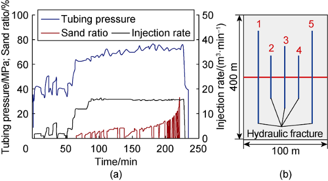
Fig. 6. Fracturing pressure data (a) and physical model of fracturing-soaking-production simulation based on data inversion (b). |
Table 5. Main input parameters in the simulation |
| Parameter | Value | Parameter | Value |
|---|---|---|---|
| Initial pore pressure | 47 MPa | Matrix porosity | 5% |
| Initial saturation | 40% | Matrix permeability | 0.3×10⁻³ μm2 |
| Initial salinity of formation water | 50 000×10-6 | Membrane efficiency | 6% |
| Initial salinity of fracturing fluid | 2000×10-6 | Effective volume diffusion coefficient | 0.36×10⁻⁹ m2/s |
| Oil phase viscosity | 8 mPa∙s | Water phase viscosity | 2 mPa∙s |
| Bottom hole pressure | 35 MPa | Gas constant | 8.314 J/(mol∙K) |
| Injection rate | 50 m³/h | Thickness of the reservoir | 40 m |
| Injection time | 30 h | Well spacing | 400 m |
| Stage length | 100 m |
Figs. 7 and 8 show the distribution of pore pressure and oil saturation at different moments in fracturing, soaking and production stages respectively. It can be seen that fracturing is a physical process similar to transient water flooding. With the increase of fracturing time, oil saturation near fractures gradually decreases while the pore pressure gradually increases. In the soaking stage, influenced by capillary pressure, chemical potential and osmotic pressure, the oil saturation near the fractures gradually recovers, and a large amount of crude oil in the matrix is displaced into the fractures, so the oil production is high at the beginning of the well opening after soaking. With the increase of shut-in time, pore pressure tends to a certain equilibrium value. Under closed boundaries, the pore pressure when the reservoir reaches equilibrium is greater than the initial pore pressure. In production stage, the simulation results of pore pressure and oil saturation show the same trends as in conventional production process.
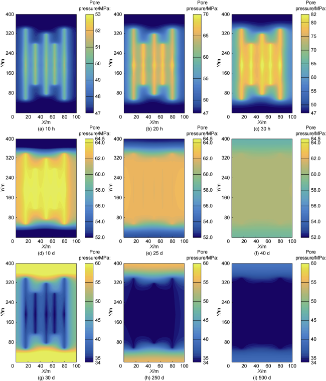
Fig. 7. Pore pressure distribution at different moments in fracturing (a-c), soaking (d-f) and production (g-i) stages. |
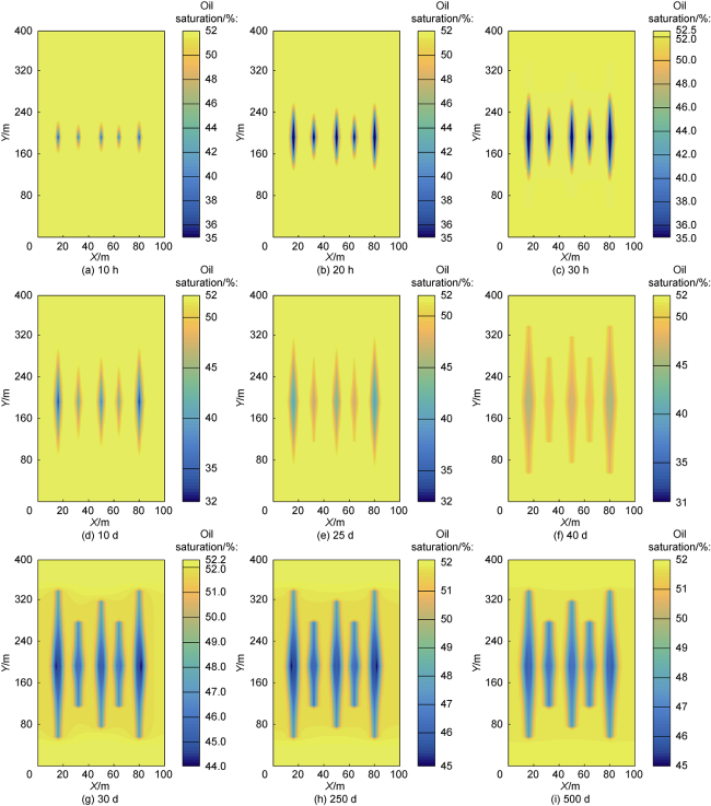
Fig. 8. Oil saturation distribution at different moments in fracturing (a-c), soaking (d-f) and production (g-i) stages. |
By changing the shut-in time, the production performance curves at different shut-in moments were simulated (Fig. 9 a). Taking the cumulative production of 300 d into production without shut-in as the reference, the relationship between the soaking time and the cumulative production increment is shown in Fig. 9 b. Fig. 9 a shows that the initial daily production and cumulative production increased significantly after shut-in, but the increase of the cumulative production decreased with the increase of production time. Fig. 9 b shows that with the increase of shut-in time, the cumulative production increment increased first and then gradually approached a stable value. In order to reasonably control shut-in time, produce crude oil and recover the cost as soon as possible, according to the shut-in time optimization method, the point with curve slope of 0.001 t/d in Fig. 9 b was found, and the corresponding value of 50 d was the optimal shut-in time.
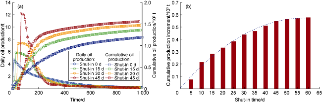
Fig. 9. Production dynamics (a) and cumulative production increment (b) at different shut-in times. |
4. Analysis of influencing factors of optimal shut-in time
Based on the integrated fracturing-soaking-production model and the physical model shown in Fig. 6 b, the influences of matrix permeability, porosity, membrane efficiency, capillary pressure multiple, displacement rate, total injected liquid volume and fracture length on the optimal shut-in time were studied. When analyzing the influence of a parameter, only different values were set for this parameter. The values of other parameters were the same as those in the above example.
4.1. Influences of matrix permeability and porosity on optimal shut-in time
The relationship curves between matrix permeability and porosity with optimal shut-in time were obtained from simulation as shown in Fig. 10 , and the corresponding regression relationships were given. Influenced by the transport rates of oil, water and solute in the matrix, the optimal shut-in time has a logarithmic decreasing relationship with matrix permeability and a weakly nonlinear decreasing relationship with porosity. The matrix permeability with lower values has a significant effect on the optimal shut-in time.
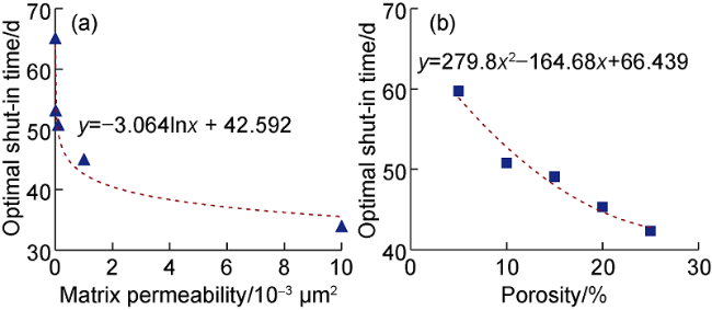
Fig. 10. Relationship curves between optimal shut-in time wtih matrix permeability (a) and porosity (b). |
4.2. Influences of membrane efficiency and capillary pressure multiple on optimal shut-in time
Membrane efficiency and capillary pressure have great influence on imbibition between matrix and fracture under water-wet condition. The influences of membrane efficiency and capillary pressure multiple (the ratio of the current capillary pressure to the initial capillary pressure) on the optimal shut-in time were examined, and the results are shown in Fig. 11 . The optimal shut-in time is in non-linear positive correlation with membrane efficiency and non-linear negative correlation with capillary pressure multiple. With the decrease of membrane efficiency and the increase of capillary pressure multiple, the water phase in the fracture will enter the matrix to replace the oil phase more easily, and the oil saturation near the hydraulic fracture will recover more quickly, and the reservoir will reach equilibrium state more quickly.
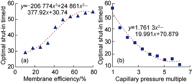
Fig. 11. Relationship curves between optimal shut-in time with membrane efficiency (a) and capillary pressure multiple (b). |
4.3. Influence of displacement rate, total liquid injection volume and fracture length on optimal shut-in time
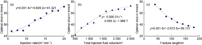
In fracturing, displacement rate, total injected liquid volume and fracture length are key parameters affecting the fluid distribution pattern after injection, and also key parameters affecting the optimal shut-in time. The influences of displacement rate, fracture length and total injected liquid volume on optimal shut-in time were investigated, and the simulation results are shown in Fig. 12 . In the influence analysis of fracture length, the physical model had 5 clusters of fractures with equal cluster spacing and length. The optimal shut-in time shows a nearly linear positive correlation with displacement rate, a nonlinear positive correlation with the total injected liquid volume, and a nonlinear negative correlation with fracture length. With the same amount of fracturing fluid injected, the increase of displacement rate makes the time of high pressure injection reduce, and more fracturing fluid remains in the hydraulic fractures after stop of pumping, forming local high pressure area. In this case, longer soaking time is needed for energy and multiphase fluid flow in the reservoir to reach balance. The increase of the total injected liquid volume directly increases the absorption load of the reservoir. According to the law of mass conservation and the mass transfer equation in porous media, when the mass transfer capacity of fracture and matrix remains unchanged, the increase of total injected liquid volume inevitably leads to the increase of mass transfer time. The decrease of fracture length makes the area of oil/water imbibition exchange between matrix and fracture decrease, thus increasing the optimal shut-in time.
Fig. 12. Relationship curves between displacement rate (a), total injected liquid volume (b), fracture length (c) with optimal shut-in time. |
4.4. Controlling factors of optimal shut-in time
In order to sort out the main controlling factors of optimal shut-in time, 7 influencing factors were analyzed, and the corresponding parameter settings are shown in Table 6 . Based on orthogonal design, the seven influencing factors were combined and a total of 21 modeling schemes were obtained. Based on the main input parameters in Table 5 , the results of multivariate variance analysis obtained by simulation are shown in Table 7 . It can be seen from the mean square and F values, the factors in descending order of influence on the optimal shut-in time are the total injected liquid volume, capillary pressure multiple, matrix permeability, porosity, membrane efficiency, salinity and displacement rate of fracturing fluid.
Table 6. Parameter settings of orthogonal experiments |
| Number | Parameter | Value |
|---|---|---|
| 1 | Membrane efficiency | 5%, 10%, 15% |
| 2 | Capillary pressure multiple | 1, 3, 5 |
| 3 | Total volume of liquid injected | 1000, 1500, 2000 m3 |
| 4 | Matrix permeability | 0.01×10⁻³, 0.10×10⁻³, 1.00×10⁻³ μm2 |
| 5 | Fracturing fluid salinity | 1000×10-6, 3000×10-6, 5000×10-6 |
| 6 | Porosity | 4%, 6%, 8% |
| 7 | Displacement rate | 10, 40, 70 m3/h |
Table 7. Results of multivariate variance analysis |
| Number | Parameter | Sum of squares | Degree of freedom | Mean square | F | P |
|---|---|---|---|---|---|---|
| 7 | Displacement rate | 0.048 | 2 | 0.025 | 0.357 | 0.868 |
| 5 | Fracturing fluid salinity | 0.126 | 2 | 0.063 | 0.614 | 0.577 |
| 1 | Membrane efficiency | 0.311 | 2 | 0.155 | 1.521 | 0.305 |
| 6 | Porosity | 0.336 | 2 | 0.198 | 1.942 | 0.313 |
| 4 | Matrix permeability | 0.363 | 2 | 0.281 | 3.775 | 0.262 |
| 2 | Capillary pressure multiple | 0.684 | 2 | 0.742 | 6.349 | 0.0319 |
| 3 | Total volume of liquid injected | 1.619 | 2 | 0.809 | 7.922 | 0.028 |
5. Conclusions
With the increase of shut-in time, both the initial production and cumulative production increment of shale wells increase rapidly at first and then tend to a stable value. The shut-in time corresponding to the inflection point in the trend of cumulative production increment is the optimal shut-in time.
The optimal shut-in time has a nonlinear negative correlation with matrix permeability, porosity, capillary pressure multiple and fracture length, a nonlinear positive correlation with membrane efficiency and the total injected liquid volume, and a nearly linear positive correlation with displacement rate. The factors in descending order of influence on the optimal soaking time are the total injected liquid volume, capillary pressure multiple, matrix permeability, porosity, membrane efficiency, fracturing fluid salinity and displacement rate.
Nomenclature
csm, csf—solute mass fraction in matrix and fracture, %;
csf,in,pro—solute mass fraction of sink term in fracture, %;
cswmf—solute mass fraction in the unit where fracture and matrix intersect, %;
Δcsmf—difference of solute mass fraction between matrix and fracture, %;
Cm, Cf—compressibility coefficients of matrix and fracture porosity, Pa-1;
Deff—effective volume diffusion coefficient in porous media, m2/s;
Dm—altitude, m;
Em, Ef—stress sensitivity coefficients of matrix and fracture permeability, Pa-1;
F—level of significant difference;
Km, Kf—permeability of matrix and fracture, m2;
K0,m, K0,f—initial permeability of matrix and fracture, m2;
n—fracturing stages;
p0—initial pore pressure, Pa;
pc—capillary pressure, Pa;
pof, pwf—pressures of oil phase and water phase in fracture, Pa;
pom, pwm—pressures of oil phase and water phase in matrix, Pa;
Δpomf, Δpwmf—pressure differences of oil phase and water phase between matrix and fracture, Pa;
Δpop—osmotic pressure difference, Pa;
P—detection level;
qof, qwf—source and sink terms of oil and water phases in fractures, s-1;
qomf, qwmf, qsmf—exchange terms of oil phase, water phase and solute between matrix and fracture, s-1;
R—gas constant, J/(mol·K);
Sof, Swf—saturation of oil phase and water phase in fracture, %;
Som, Swm—saturation of oil and water phases in the matrix, %;
t—time, s;
Tm—temperature of matrix, K;
Tomf, Twmf—conductivity coefficients of oil phase and water phase between matrix and fracture based on embedded discrete fracture model, m3;
Vm—grid cell volume, m3;
Vw—partial molar volume of water, m³/mol;
X, Y—rectangular coordinate system, m;
γo, γw—API gravity of oil phase and water phase, N/m3;
εvm—volume strain, dimensionless;
λof, λwf—relative fluidity of oil phase and water phase in fracture, (Pa•s)-1;
λom, λwm—relative fluidity of oil phase and water phase in matrix, (Pa·s)-1;
λomf, λwmf—relative fluidity of oil phase and water phase corresponding to matrix and fracture intersecting unit, (Pa·s)-1;
ρw, ρs—density of the water phase and solute, kg/m3;
ϕm, ϕf—porosity of matrix and fracture, %;
ϕ0,m, ϕ0,f—initial porosity of matrix and fracture, %;
ω—membrane efficiency, dimensionless.