

Introduction
Thin-interbedded reservoirs are widely developed in oil and gas basins in China, and are also important exploration targets for lithologic reservoirs. The accurate prediction of distribution of thin-interbedded reservoirs is of great significance. However, due to the limitation of resolution, it is difficult for seismic data to meet the needs of thin reservoir identification, which restricts the lithologic reservoir exploration seriously. In view of the technical bottleneck of seismic data resolution, scholars have carried out fruitful researches on seismic inversion method [1⇓⇓⇓⇓-6] and tuning theory [7⇓⇓⇓-11]. On the one hand, the vertical resolution has been enhanced by means of inversion, widening frequency processing methods and other processing methods to identify thin layers. On the other hand, thin layers are identified by their amplitude changes on the basis of tuning effect. For example, the minimum thickness of thin layers identifiable is 1/8 wavelength by using the amplitude tuning principle [1⇓-3]. Zeng [12-15]put forward the concept of seismic sedimentology from the perspective of lateral resolution of seismic data, and two practical technologies of -90° phase shift and stratal slicing, which can avoid the difficulty in improving vertical resolution. Subsequently, many experts and scholars conducted a large number of studies to explore its basic principles, research procedures, application conditions and potential risks [16⇓⇓⇓-20]. In recent years, many good application examples have been achieved by seismic sedimentology methods in sedimentary facies research and reservoir prediction [16,20⇓⇓⇓ -24]. Based on the basic geological understanding that the actual width is much larger than the thickness of a sedimentary body and the advantage of lateral resolution of seismic data [17,19,24], seismic sedimentology can detect distributions of thin layers much lower than the seismic resolution limit. By using this technology, Zeng et al. depicted shallow water delta distributary channels in Qijia area of Songliao Basin, NE China and even sorted out thin layers of only 1 m thick [16], showing the great potential of seismic sedimentology.
Due to the limitation of seismic data resolution and many influence factors in the application [19], seismic sedimentology is still difficult to meet the needs of practical exploration in thin-interbedded reservoir prediction. Unlike a single thin layer, single sand body in thin-interbeds is difficult to be identified accurately by seismic sedimentology method due to interference. To solve this problem, Zeng [21] proposed to use slice sequence to analyze the changes of thin interbeds and then determine the distribution of each thin layer. Li et al. analyzed the interference process of thin interbeds, and predicted thin layers by reducing the slice interval to 0.2 ms to find zero-value slices without interference [22-23]. These studies have shown that when thin interbeds are difficult to distinguish vertically, if the target slice does not have adjacent layer interference, the distribution of the target layer can still be predicted. Since each sample point in the slice of thin interbeds is the comprehensive response of multiple thin layers, when the spacing thickness of two thin layers is large enough, the interference effect of the adjacent layer is relatively weak, and the distribution of the two thin layers can be distinguished by using the previous methods effectively. When the spacing thickness of two thin layers decreases to a certain extent, the response of the target thin layer is easy to be completely concealed by the response of adjacent thin layer. In this case, it is still difficult to accurately distinguish different thin layers on the same slice by analyzing the changes of thin-interbeds and finding zero-value slices without interference.
On the basis of previous studies, we propose two methods including minimum interference frequency and superimposed slicing following the idea of directly suppressing adjacent layer interference in target layer slice. These methods can maintain accurate relative relationship between the plane amplitude, so that the target thin layer in the thin interbeds can not be distinguished vertically, but can be detected horizontally. Among them, the minimum interference frequency method uses the basic principle that the interference of the adjacent layer to the sampling point of the target layer changes with frequency, and generates stratal slices by finding the minimum frequency of interference to the target layer, then the interference of the adjacent layer can be suppressed. The superimposed slicing method reduces the influence of the interference layer in the target layer slice by stacking the interference layer slices with different weight coefficients to the target layer slice. The three-dimensional numerical model verifies the feasibility of this method. Taking Fengnan area of Junggar Basin, NW China as an example, the distribution of target sand body is predicted by the above two methods accurately, which provides a reference for the prediction of thin-interbedded reservoir distribution in continental basins.
1. Minimum interference frequency method
1.1. The meaning of minimum interference frequency
By making full use of the advantages of lateral resolution of seismic data, seismic sedimentology technology improves the prediction accuracy of thin layers greatly. Zeng et al. pointed out that geological bodies with thickness less than 1/4 wavelength can be identified by stratal slices [16]. But for thin-interbedded reservoirs, each sample point in the slice is the comprehensive response of multiple thin layers. Therefore, it is difficult to distinguish different thin layers on the same slice accurately.
When thin interbeds are vertically indistinguishable, the interference effect of adjacent thin layers on the target thin layer changes with frequency. The frequency with the smallest interference effect can be called the minimum-interference frequency. In order to explain the meaning of the minimum-interference frequency, we built a double-interface model to analyze the influence of interference on slices at different frequencies. The model description is as follows. The top interface and the bottom interface had the same reflection coefficient of 1, and were 10 ms apart from each other. The forward modeling profile (Fig. 1 a) was obtained by convolution of 5-100 Hz zero phase Ricker wavelet, and then the amplitude values at the red line position (50 ms) were extracted to plot the curve of amplitude with changing frequency (Fig. 1 b). It can be seen from Fig. 1 that the amplitude decreases with the increase of frequency less than the peak value, indicating that the interference effect of the bottom interface on the top interface is weakening. When the amplitude decreases to the blue dotted line (at the frequency of 22 Hz), the amplitude value is the same as that at the maximum frequency, indicating that the interference value of the bottom interface at this sampling point is zero, and the corresponding frequency is called the minimum-interference frequency. In order to further illustrate the meaning of minimum-interference frequency, forward seismic traces were obtained by convolution of 22 Hz zero phase Ricker wavelet with the top interface, bottom interface and top-bottom double interface (Fig. 2 ). It can be seen from Fig. 2 that at the time position of the top interface, the amplitude of the bottom interface reflection (blue line) is zero, and the amplitude of the top interface reflection (red line) is the same as that (intersection point) of the double interface reflection (black line), indicating that the bottom interface reflection does not interfere with the sampling point. If we extract the amplitude slice of the top interface position at this corresponding frequency, the top interface is not affected by the bottom interface and can be detected horizontally. Except the sampling point corresponding to the top interface, the bottom interface has interference on all the other sampling points, so the top and bottom interfaces are still unable to be distinguished in the comprehensive response profile.
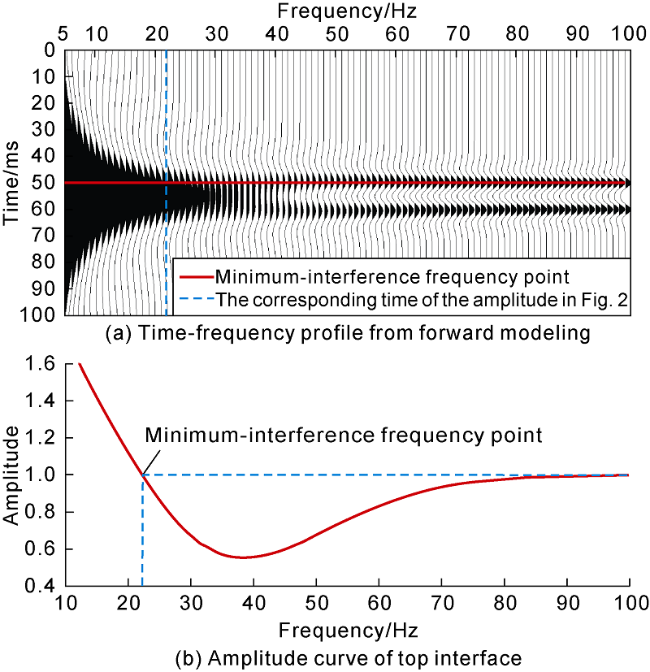
Fig. 1. Forward modeling of double-interface model. |
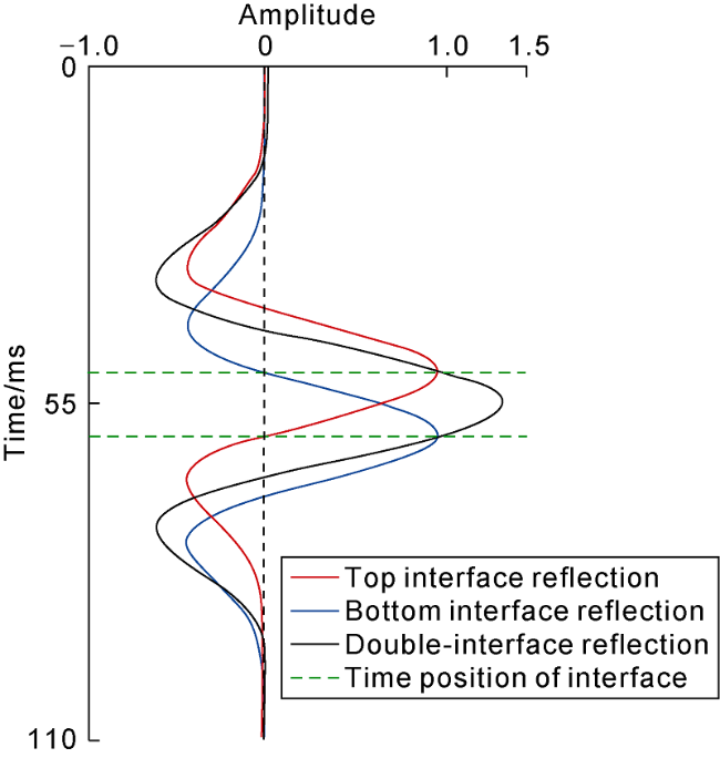
Fig. 2. Interference process of double-interface model. |
If the seismic response formed by the -90° phase shift wavelet of a single thin layer is regarded as a composite wavelet, the interference effect of two thin layers is similar to that of the double-interface model in ideal state. When the amplitude of the composite wavelet formed by adjacent thin layers at the center point of the target thin layer is zero, the corresponding frequency is called the minimum-interference frequency. Therefore, in the case of two thin layers, if the minimum-interference frequency of the interference layer to the target thin layer is determined, the stratal slice of the target layer extracted at this frequency will have much less interference of the adjacent layer and highlight the target thin layer effectively. In this case, although the target thin layer can not be distinguished on the profile, it can be detected on the plane.
For the case with three thin layers, the target layer has two interference layers, and each interference layer has a minimum-interference frequency for the target thin layer. If the two minimum-interference frequencies are close, the above method is still effective. When the interference layers exceed two, it is difficult to find an optimal frequency close to the minimum-interference frequency of each interference layer. Therefore, this method is applicable to the cases with less than 3 thin layers only.
1.2. Determination of minimum interference frequency
The minimum-interference frequency is closely related to the composite wavelet, thin layer thickness and interlayer thickness. The composite wavelet is affected by the wave impedance difference of surrounding rocks. At different wave impedance differences of surrounding rocks, the wavelet frequency and thin layer thickness will also affect the composite wavelet. Therefore, it is very difficult to confirm the minimum-interference frequency directly. Su et al. [18-19] pointed out that the -90° phase shift data volume converted from seismic data had a better correspondence between the waveform and the thin layer. In theory, a single thin layer corresponds to the peak position on the -90° phase shift profile. It can be seen from Fig. 2 that the amplitude of the top interface at the minimum-interference frequency is close to the peak. According to this phenomenon, in practical application, the minimum-interference frequency can be made out according to the amplitude-frequency characteristics (AVF) of the seismic data through the well, that is, we can look for the frequency corresponding to the center of the thin layer close to the upper or lower edge of the peak.
Real data in the work area was analyzed. Well W1 is a typical well in the work area, which has encountered three thin reservoirs of 6, 6 and 8 m thick respectively. The mudstone layers between the reservoirs are 8 m and 16 m thick, respectively. The middle thin reservoir is the oil-bearing layer. The dominant frequency of seismic data is about 40 Hz and 10-60 Hz in bandwidth. The reservoirs on logging curves feature generally low natural gamma, high self-potential and high wave impedance, in which the oil layer has slightly lower self-potential and wave impedance than the two adjacent reservoirs. The seismic wave velocity of the target sandstone layer is about 4000 m/s. According to 1/4 wavelength, the minimum sandstone thickness identifiable is about 25 m, which is much larger than the reservoir thickness. The three sets of reservoirs have small thickness, close spacing and serious mutual interferences, making it difficult to distinguish them on seismic profile.
Wavelet transform can be used to amplify and transpose signals and extract features of the signals, and is also used for multi-resolution analysis to achieve separation of high and low frequencies. Therefore, wavelet transform was adopted to work out the minimum-interference frequency and extract subsequent slices in this work. Fig. 3 shows the amplitude-frequency characteristics extracted from -90° phase shift data volume of Well W1 based on wavelet transform. It can be seen from Fig. 3 a that the thin layers have good correspondence with waveform mostly, but the oil layer is located at the zero point between the peak and through, indicating that the oil layer may be affected by interference of adjacent thin layers. As the frequency increased gradually from 40 Hz, the amplitude of the target layer was still close to the zero point. Therefore, increasing frequency within the effective frequency bandwidth range could not reduce the interference of the adjacent layers, and the target layer is still difficult to be made out on the profile effectively. When the frequency was gradually reduced from 40 Hz, the amplitude of the target layer rapidly approached the peak amplitude. When the frequency was 20 Hz, the target layer was close to the amplitude center, indicating that the adjacent layers might have smaller interference on the target layer. In order to illustrate amplitude changes of the oil layer with frequency more clearly, the amplitude curve corresponding to the oil layer section of Fig. 3 a (horizontal blue dotted line) was extracted (Fig. 3 b), with the peak frequency of about 26 Hz. The relative relationship between the minimum-interference frequency and the peak frequency is similar to the theoretical situation (Fig. 2 ). Therefore, 20 Hz might be the minimum-interference frequency of the target layer.
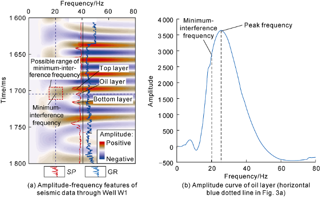
Fig. 3. Amplitude-frequency features of seismic data of Well W1 based on wavelet transform. |
The minimum-interference frequency was verified by simulating the interference process of three sets of reservoirs in Well W1. Firstly, the acoustic curve was divided into three sections corresponding to the three thin reservoirs, and then synthetic seismic records were obtained by using -90° phase shift Ricker wavelet of 20 Hz and 40 Hz frequency without changing the travel time of seismic wave (Fig. 4 ). Trace c and Trace d are the acoustic curve and synthetic record of the middle oil layers. It can be seen from the Trace d that the amplitude of the oil layer center was the maximum peak (points B1 and B2) no matter the wavelet frequency was 20 Hz or 40 Hz, but the interferences of the adjacent thin layers on the target layer changed with frequency. When the frequency was 20 Hz, the interference of the adjacent thin layers to the target layer was close to zero (points A1 and C1), and the amplitude of the oil layer (point D1) was close to the peak amplitude. When the frequency was 40 Hz, the adjacent thin layers had relatively strong interference to the target layer (points A2 and C2). The negative interference values counteracted the amplitude values of the target layer, so the amplitude of the target layer was close to zero (point D2). Therefore, the synthetic record of Well W1 verifies that 20 Hz is close to the minimum-interference frequency of the top and bottom interference layers to the target layer.
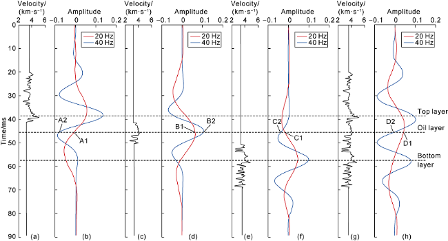
Fig. 4. Synthetic seismic records by -90° phase shift Ricker wavelet (20 Hz and 40 Hz) of the three thin reservoirs in Well W1. Trace a and Trace b are the acoustic curve and synthetic record of the top thin layers.Trace c and Trace d are the acoustic curve and synthetic record of the middle oil layers. Trace e and Trace f are the acoustic curve and synthetic record of the bottom thin layers. Trace g and Trace h are the whole acoustic curve and synthetic record. The black dotted line is the center time of the target layer. |
There are 9 wells in this work area, where only Well W1 was selected to calculate the minimum-interference frequency. As the reservoirs in the study area have small changes in transverse thickness, the same conclusion can be obtained by using other wells to look for the minimum- interference frequency. The scanning results of wavelet frequency-division amplitude slices from 16-30 Hz also show that the results extracted at 20 Hz had the clearest characterization of the channel and the highest coincidence rate with drilling data. This proves from another perspective that 20 Hz is the frequency closest to the minimum interference for both the top layer and the bottom layer.
2. The superimposed method based on stratal slice
2.1. Technical principle
A double-layer model (Fig. 5 ) is taken as example to explain the principle of superimposed slice. Assuming the amplitude of different regions in Slice A as a0, a1 and a2, and the amplitude of different regions in Slice B as b0, b1 and b2 respectively. Then the amplitude a2 and b2 of overlap region equal to the sum of the amplitude of this layer and the amplitude from adjacent layer interference, that is:
$\left\{ \begin{align} & {{a}_{2}}={{a}_{0}}+{{a}_{1}} \\ & {{b}_{2}}={{b}_{0}}+{{b}_{1}} \\ \end{align} \right.$
The amplitude ck of any point on the superimposed slice of thin layer B is defined as:
ck=bk-w0ak
where ${{w}_{0}}=\frac{{{b}_{0}}}{{{a}_{0}}}$
By substituting Eq. (1) into Eq. (2), we can obtain the points with amplitude of b1 and b2 in the Slice B have the same amplitude of (b1-w0b0) in superimposed slice, and the point with the amplitude of b0 has zero value in the superimposed slice. The superimpose area and non-interference area of thin layer B have the same amplitude, and the relative relationship is the same as that of single thin layer, indicating that superimposing slices can suppress adjacent layer interference effectively.
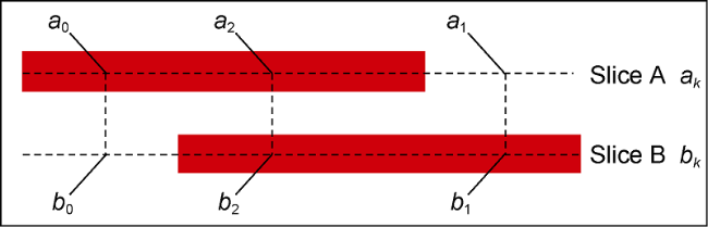
Fig. 5. The two-layer model |
Similarly, we can obtain the interference coefficient of each interference layer corresponding to the target layer slice in the case with multiple thin layers. The calculation formula is as follows:
$\left[ \begin{matrix} {{a}_{00}} & \cdots & {{a}_{0j}} & \cdots & {{a}_{0,n-1}} \\ \vdots & {} & \vdots & {} & \vdots \\ {{a}_{i0}} & \cdots & {{a}_{ij}} & \cdots & {{a}_{i,n-1}} \\ \vdots & {} & \vdots & {} & \vdots \\ {{a}_{n-1,0}} & \cdots & {{a}_{n-1,j}} & \cdots & {{a}_{n-1,n-1}} \\\end{matrix} \right]\left[ \begin{matrix} {{w}_{0}} \\ \vdots \\ {{w}_{i}} \\ \vdots \\ {{w}_{n-1}} \\\end{matrix} \right]=\left[ \begin{matrix} {{b}_{0}} \\ \vdots \\ {{b}_{i}} \\ \vdots \\ {{b}_{n-1}} \\\end{matrix} \right]$
The calculation formula of superimposed slice in the case with multiple thin layers is:
${{c}_{j}}={{b}_{j}}-\sum\nolimits_{i=0}^{i=n-1}{{{w}_{i}}{{a}_{ij}}}$
In the case that the layers are stable in thickness, if a non-interference area can be found in each interference layer, the relative relationship of amplitude of the target layer and each interference layer can be determined, then the interference coefficient of each interference layer can be calculated, and finally the product of the amplitude of each interference layer with the interference coefficient is stacked on the target slice to form superimposed slice. The superimposed slice can suppress the interference of adjacent layers effectively and keep the relative relationship of amplitude of the target layer.
2.2. Method validation
In order to verify the rationality of the superimposed method based on stratal slicing and identification ability to thin interbeds of this method, a forward model of thin interbeds was built for superimposed slice experiment.
Parameters of the three-dimensional model are as follows: there were four thin sand bodies in the mudstone background, and the plane distribution of each sand body is shown in Fig. 6 a. We extracted the corresponding profile of the red line to get the vertical distribution of the sand body (Fig. 6 b). The sandstone layers and mudstone interlayers were both 4 m thick. The velocities of the four sandstone layers from bottom to top were 3600, 3800, 4200 and 4000 m/s respectively, and the velocity of the background mudstone was 3000 m/s. The profile was obtained by forward modeling of -90° phase shift of 40 Hz Ricker wavelet (Fig. 6 c), and the four thin sand bodies cannot be distinguished completely on the seismic profile.
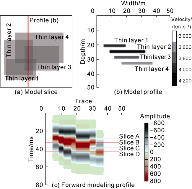
Fig. 6. 3D model of the 4 layers and forward modeling profile. |
The stratal slices corresponding to the four thin sand bodies are shown in Fig. 7 a-7d. The distribution of the thin sand bodies on each slice is not so clear and complete. The fourth layer slice is taken as an example to illustrate the calculation process of superimposed slice. For the fourth thin sand body interfered by the adjacent three thin sand bodies, first the non-interference points of the other three slices were sorted out (blue points in Fig. 7 a-7c), and the amplitude values of each layer slice corresponding to the three non-interference points were extracted. Then, the interference coefficient of each layer slice was calculated with Eq. (3). Finally, the stacked slice of the sand body of fourth layer was obtained according to Eq. (4). Similarly, stacked slices of the other three layers were obtained as shown in Fig. 7 e-7h. Compared with the conventional stratal slices, the superimposed slices show more clearly the distribution of the thin sandbody, with the adjacent layer interferences well suppressed.
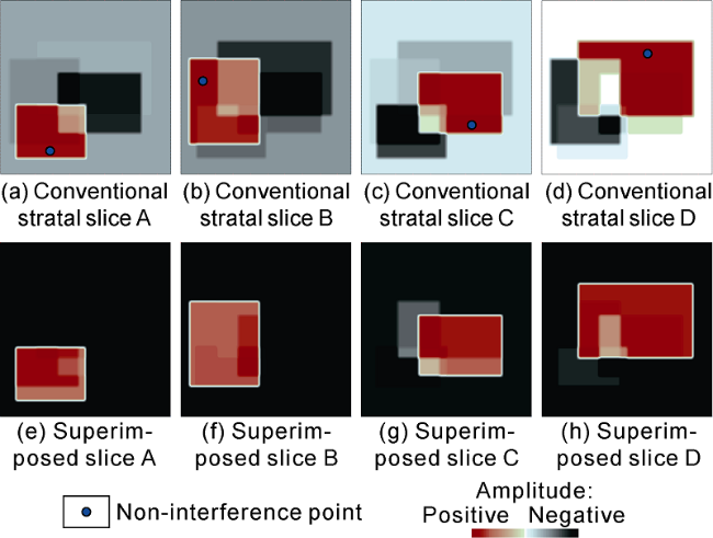
Fig. 7. Conventional stratal slices and superimposed slices. |
2.3. Analysis of influence factors
There are many factors affecting the results of superimposed slice, including the selection of interference layer slice and non-interference point, the change of formation thickness, the influence of isochronism, the amplitude fidelity of seismic data and so on. Among them, the influences of relative isochronism of slice and amplitude fidelity of seismic data are universal, so they aren’t discussed in this paper. The other three factors that have special influence on the results of superimposed slice were analyzed.
The selection of interference layer slice is a major factor affecting the result of superimposed slice. In theory, each interference layer slice needs to be stacked on the target layer slice to suppress the interference of adjacent layers. But in practical applications, it is difficult to determine the number of interference layer slices. Therefore, it is necessary to explore whether stacking part of interference layer slices can improve the slicing effect.
Taking the fourth layer slice of Fig. 7 d as an example, a conventional stratal slice (Fig. 7 a-7c) was stacked respectively, and partially superimposed slices obtained are shown in Fig. 8 a-8c. Among them, Fig. 8 a and Fig. 8 c have poor results after stacking, while Fig. 8 b is better. Compared with the total superimposed slice (Fig. 8 d), it can be seen that the sand body of the partially superimposed slice is well characterized, but the mudstone background is not well suppressed. The reason is that the conventional slice B is the main factor affecting the integrity of the fourth layer sand body. Therefore, to be effective, the superimposed slicing method only needs to stack the key slices that affect the complete characterization of sand body morphology in the target layer rather than stack all the slices that interfere with the target sand body.
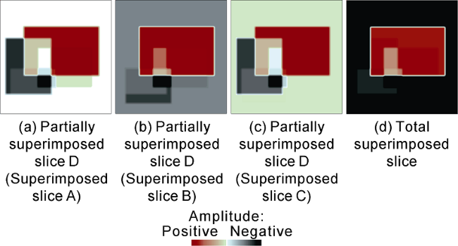
Fig. 8. Partially superimposed slices with different conventional slices and total superimposed slice. |
The selection of non-interference points is another important factor affecting the result of superimposed slice. Taking the fourth slice with only the conventional slice B stacked as an example, different non-interference points were used to calculate the partially superimposed slices (Fig. 9 a-9d). The four slices all use wrong non- interference points. It can be seen that the sand bodies in Fig. 9 a and Fig. 9 b are still more clear and complete than that of the original stratal slice. Compared with the calculation results with correct non-interference point (Fig. 8 b), they have more obvious mudstone background. With non-interference points selected in the distribution range of the sand bodies, Fig. 8 c and 8d show no obvious effect of stacking. The above analysis shows that when the non-interference points selected are outside the sand body distribution, even if the points selected are wrong, the result of superimposed slice can still be improved.
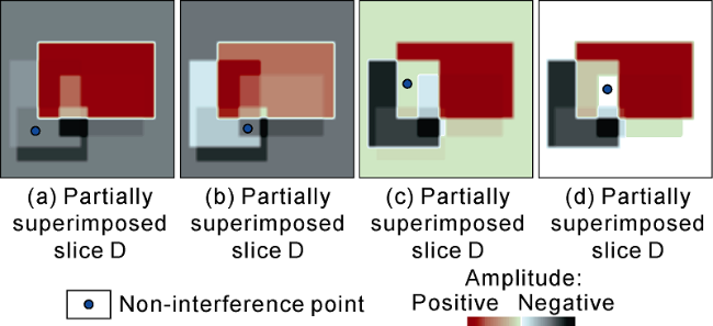
Fig. 9. Partially superimposed slices obtained by selecting different non-interference points. |
The superimposed slice method is based on the assumption of constant formation thickness. A three-dimensional model with layers changing insignificantly in thickness was built to explore whether the superimposed slice is still effective in the case of layers with small thickness changes. The model parameters were as follows (Fig. 10 ).There were five sets of thin sand bodies under the mudstone background in the model. The sand bodies were 4 m thick, the mudstone interlayers were 1-6 m thick, the velocity of background mudstone was 2700 m/s, the velocity of non-target sandstone layers was 2800 m/s, the velocity of target sandstone layer was 3500 m/s, and the maximum layer thickness change in the model was 22 m. 30 Hz Ricker wavelet with -90° phase shift was used to do convolution to obtain the forward profile as shown in Fig. 10 b. The five sets of sand bodies cannot be identified on the profile. Fig. 10 h-10l shows the extracted conventional stratal slices. It can be seen from them that the sand bodies distribution can’t be clearly distinguished. Fig. 10 m-10q shows the extracted superimposed slices. Although there are still shadows of other layers of sand bodies, the distribution of target sand body is completely depicted, proving that for the case with small thickness changes of layers, the superimposed slice can still suppress the interference of adjacent layers and highlight the distribution of target reservoir.
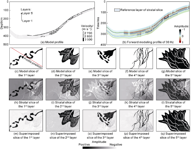
Fig. 10. Comparison of stratal slices and superimposed slices of three-dimensional model of different thickness formations in the study area. |
3. Case study
3.1. Geological overview and well-seismic data conditions of the study area
The study area is located in Mabei slope area of Mahu area at northwestern margin of Junggar Basin (Fig. 11 ), and the target layer is the upper member of Triassic Karamay Formation. According to previous studies, the Karamay Formation in Mahu area is mainly composed of braided river delta deposits, in which the reservoirs are mainly delta front underwater distributary channel sand bodies. In this work, distribution of oil-bearing layers in Well W1 was examined, and the seismic data used was the same as that in Section 1.2.
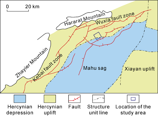
Fig. 11. Location of the study area. |
The cross-well sand layer correlation (Fig. 12 ) shows that sand bodies in the study area feature vertical superposition, thin thickness and fast lateral change. The cross well seismic profile after -90° phase shift (Fig. 13 ) shows that the oil layer is close to the zero point. The top layer and bottom layer have good correspondence with the peak of event and good continuity. Similar to adjacent wells, oil layers in Well W1 are difficult to distinguish on the seismic profile. Due to thin reservoir thickness and small wave impedance difference between tight sandstone and favorable sandstone reservoir, it is difficult to predict single sand body in this well by conventional methods effectively. Therefore, the inversion method was tried to predict the plane distribution of the oil layers. By comparing the results of wave impedance inversion, waveform indication inversion and waveform indication simulation, it is found that the results of wave impedance inversion cannot distinguish the oil layers from interference layers, and the results of waveform indication simulation have poor continuity (due to the limited space, only the waveform indication inversion results with good effect are shown in this paper). Through parameter tests of different curves, the self-potential curve with obvious response to the sand bodies was selected as the characteristic curve, and all 9 wells were involved in the inversion. The cross well inversion profile (Fig. 14 a) shows that the oil layer and the top and bottom interference layers in Well W1 can be well distinguished. The plane attribute of inversion result (Fig. 14 b) shows that point W6 is inconsistent with the drilling results, while the other points are in good agreement with the drilling results. But the plane results show no geological regularities, which are inconsistent with the geological understanding of underwater distributary channels.
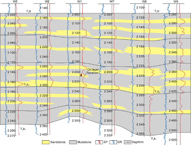
Fig. 12. Cross-well sand layer correlation in the study area. T2k—Middle Triassic Karamay Formation, T3b—Upper Triassic Baikouquan Formation. |
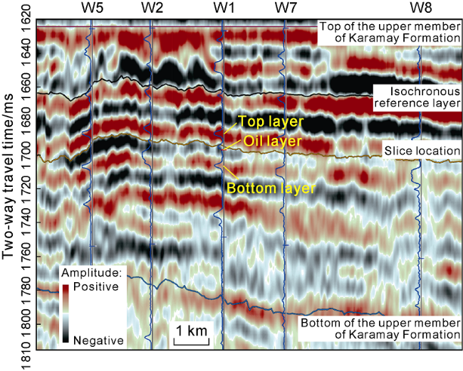
Fig. 13. Cross-well seismic profile of -90° phase shift in the study area. |
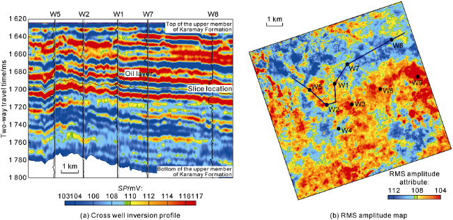
Fig. 14. Profile and plane map of the waveform indication inversion results in the study area. |
3.2. Application of minimum-interference frequency slice
In section 1.2, the minimum-interference frequency of the target layer has been determined at 20 Hz. In order to verify whether the 20 Hz frequency division slice data can suppress the interference of adjacent layers effectively and reflect the distribution of the target oil layer, based on the research idea of Zeng et al. [16], we selected the isochronous layer between the bottom and top of the upper member of Karamay Formation with short distance to the target layer and stable event as reference layer. The -90° phase shift data was processed by 20 Hz wavelet frequency division to generate the stratal slice data volume, and then the slice of the target layer was extracted (Fig. 15 b). This figure shows the self-potential curve and natural gamma curve of 9 wells encountering the target formation. In this example, the high self-potential value represents sandstone, and the low self-potential value represents mudstone. Compared with drilling results, only wells W7 and W3 are inconsistent with drilling results. In the conventional slice of the target layer extracted directly from the -90° phase shift data volume (Fig. 15 a), five wells were inconsistent with the drilling results, with a low coincidence rate of 44%. The minimum-interference frequency slice indicates that Well W7 did not drill into the sand body of the target layer, while Well W3 drilled into the sand body. Both the wells were located at the edge of the river, so it is speculated that the reason of the inconsistency may be the diachronism of slice. Therefore, the slice of 2 ms above the target layer was extracted and compared with the slice of the target layer, and the target area was zoomed in (Fig. 16 ). The Well W7 is consistent with the new slice, while Well W3 has little change. It is inferred through analysis that the Well W3 has more than 3 thin layers, leading to incomplete interference suppression of adjacent layers.
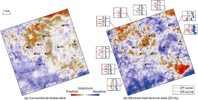
Fig. 15. Conventional slice and minimum interference slice (20Hz) of the study area. |
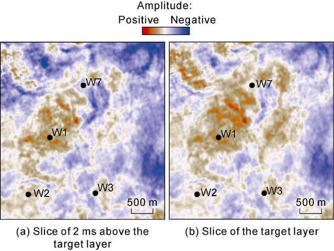
Fig. 16. Comparison of the minimum interference slice 2 ms above the target layer and target layer slice of the study area. |
The practical application shows that the actual seismic response of the target layer is concealed due to the interference of the adjacent layers on the target layer, so the conventional slice can not reflect the distribution of the target layer. In the minimum interference frequency slice, the interference of the adjacent layers is partially suppressed, and the drilling results of some wells are inconsistent with the sand bodies reflected by the slice. There are many factors may affect the suppression results, including the thickness change of the interlayer, the number of thin interbeds, the isochronism of the slice, the selection of the minimum-interference frequency.
3.3. Application of superimposed method based on stratal slice
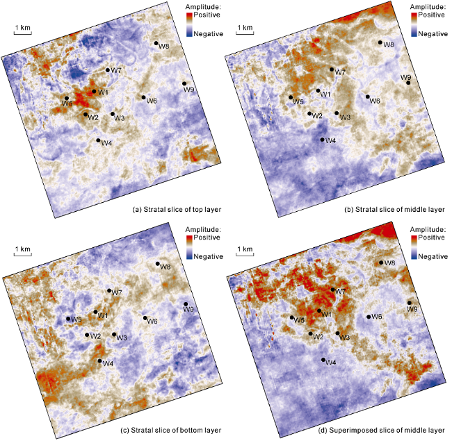
The interference of the top and bottom sets of sand bodies is the main factor making the target sand body difficult to be identified on the slice. Therefore, the conventional stratal slices corresponding to the top, middle and bottom of the three sets of sand bodies were extracted from the -90° phase shift data volume (Fig. 17 a-17c), and then the position of the non-interference point was sorted out based on the relative amplitude relationship of the same area in the three slices. That is to say, the non-interference point is the largest in amplitude on the slice and close to the peak on profile. The amplitudes of the non-interference point in the other slices need to be judged according to the distances between the slices, and are small and not located near the peak. In practical application, the search range can be narrowed by elimination method. For example, the amplitude of Well W1 in this case is close to the peak position in Fig. 17 a and 17c, indicating that there are at least two thin layers at this point. It is difficult to find the true non-interference point in practical data, but the theoretical model in section 2.3 shows that superimposed slice is still effective in suppressing adjacent layer interference as long as the non-interference point is located within the target layer. In this case, three slices were used to generate superimposed slice of the middle layer as shown in Fig. 17 d. Compared with the minimum- interference frequency slice (Fig. 15 b), the superimposed slice has lower coincidence rate with drilling results than the minimum-interference frequency slice. Compared with the conventional stratal slice (Fig. 15 a), the two key wells W1 and W2 encountering the target layer have higher coincidence rates with the superimposed slice. The overall distribution of the river channel in the superimposed slice is similar to that reflected by the minimum-interference frequency slice, but is more clear. The low coincidence between the drilling results of wells in the periphery of the river channel and the sandbodies reflected by the superimposed slice may be caused by unsatisfactory suppression of the adjacent layer interference of the superimposed method. Many factors affect the suppression results, including the selection of two important parameters of interference layer and non-interference area, the assumption of constant formation thickness, and the isochronism of formation slice etc.
Fig. 17. Stratal slices of the three sets of sand bodies and the superimposed slice of the middle target layer in the study area. |
4. Conclusions
In this study, following the research idea of suppressing adjacent layer interference by processing stratal slice, we have proposed two prediction methods for thin-interbedded reservoir distribution based on seismic sedimentology, realizing the purpose of delineating the distribution of single sand body in thin interbeds on the plane when it is difficult to distinguish the thin reservoirs on the profile. (1) In the minimum-interference frequency slicing method, the amplitude-frequency characteristics of wavelet transform are used to find the frequency with the smallest interference on the target slice, and then the stratal slice at the minimum-interference frequency is extracted. (2) In the superimposed method based on stratal slices, the interference coefficients of interference layers are calculated, the superimposed slice of the target layer is obtained by stacking the adjacent layers to the slice of target layer according to their interference coefficients.
Model test and practical application show that both of the methods can suppress the adjacent layer interference in the target slice and detect the distribution of single sand body in the thin interbeds effectively. Both of them are based on the assumption of relatively constant formation thickness. With gradual decrease of the layer thickness, it is speculated that the results of interference suppression by the two methods will be gradually deteriorated, leading to predicted boundary smaller than the actual boundary, but the overall shape of the geological body can be still predicted. Their applications to actual seismic data also show that both of the methods can predict the distribution of thin layers effectively in the case with little change of layer thickness.
The two methods have their own advantages and disadvantages. As each interference layer has a minimum interference frequency, it is difficult for the minimum-interference frequency slicing method to take into account each interference layer in the case with multiple thin layers. Therefore, this method is suitable for distribution prediction of thin-interbedded reservoirs with less than 3 layers. Although the superimposed method based on stratal slices has no limitation on the number of thin layers, each stack may introduce new errors. Therefore, the number of thin layers should not be too large. In practical application, both methods can be tried to improve the accuracy of thin layer prediction by mutual corroboration.
Nomenclature
a0, a1, a2—amplitude values of different regions in slice A;
aij—the amplitude of the jth interference point in the ith interference layer slice, when i=j, the amplitude is that of the non-interference point of the interference layer slice of the ith layer;
aj—amplitude value of point j in interference layer slice;
ak—amplitude of point k in slice A;
b0, b1, b2—amplitude values of different regions in slice B;
bj—amplitude value of point j in the target layer slice;
bk—amplitude of point k in slice B;
cj—amplitude value of point j in the superimposed slice;
GR—natural gamma, API;
i—slice mark number corresponding to the interference layer;
j—non-interference point mark number in the interference layer slice, the interference point corresponding to the adjacent slice;
n—number of interference layers;
SP—natural potential, mV;
w0—the interference coefficient of slice A to slice B;
wi—interference coefficient of ith interference layer slice.