

Introduction
To address the issues of equipment wear, sand plugging, and limited propped fracture lengths associated with existing fracturing materials [1⇓-3], Zhang et al. [4] developed a temperature-sensitive Phase-transition Fracturing Fluid System (PFFS) and proposed the self-propping phase- transition fracturing technology. PFFS consists of a Phase-transition Fluid (PF) and a Non-Phase-transition Fluid (NPF). When the temperature is below the phase- transition threshold, PFFS remains in a liquid state, allowing for easy injection and penetration into deep fractures. When the temperature exceeds the phase-transition threshold, the NPF remains liquid, while the PF undergoes a phase transition to generate In-situ self-Generated Proppant (IGP).
The phase transition process of PF highlights that temperature is critical to the successful implementation of self-propping phase-transition fracturing [5]. During the phase transition, heat is released, raising the temperature, while the low-temperature PFFS cools the formation and fractures, altering the temperature field of the formation and fractures. Therefore, it is necessary to predict the fracture temperature field under the influence of phase-transition heat, providing a basis for optimizing PFFS formulations and construction parameters. Extensive research has been conducted on the fracture temperature field during fracturing processes. Li et al. [6], based on the heat conduction equation of rock masses, established a thermal-fluid-solid coupling model. Their study suggested that temperature stress caused by the cooling effect of CO2 flow in fractures facilitates the formation of complex fracture networks around the main fracture. Seth et al. [7] developed a numerical model for calculating fracture temperatures during hydraulic fracturing and shut-in periods, investigating the effects of fracture length and rock physical properties on temperature. Guo et al. [8] considering the effects of temperature, pressure, and CO2 volumetric work, established a temperature distribution model for acid fracturing in carbonate reservoirs. Their calculations indicated that acid-rock phase-transition heat could raise fracture temperatures by approximately 15 °C.
Since the chemical reactions involved in the PF phase transition are organic reactions among its internal components, existing research results on acid-rock phase- transition heat cannot be directly applied to self-propping phase-transition fracturing technology. It is necessary to establish a reaction kinetics model for the PF phase transition to clarify the relationships of phase-transition heat with temperature and time, and to elucidate the influence of phase-transition heat on the fracture temperature field. To this end, this paper first uses the test results from Differential Scanning Calorimetry (DSC) to establish a reaction kinetics model. On this basis, according to the law of conservation of energy, a mathematical model for the temperature distribution in the formation and fractures during the fracturing process is established. A solution method is proposed, and the reliability of the model is verified. Finally, through numerical experiments, the effects of phase-transition heat, PF volume fraction, and specific heat capacity on the fracture temperature are investigated.
1. Reaction kinetics model and temperature field model
A phase-transition reaction kinetics model was established using the heat flux curves measured from DSC experiments, forming a mathematical relationship between heat release rate, temperature, and time. Based on this, a mathematical model for the temperature field of the formation and fractures, accounting for the heat from chemical phase transitions, was constructed.
1.1. Reaction kinetics model of PF
The heat flux of PF during the phase transition process was tested using a DSC Q20 apparatus. The experiment was conducted in a high-purity nitrogen environment with a flow rate of 50 mL/min. The experimental procedure was as follows: (1) Approximately 10 mg of PF sample was weighed and placed into an aluminum crucible, which was quickly sealed and loaded into the DSC sample chamber. (2) A sealed empty aluminum crucible was placed in the DSC sample chamber as a reference. (3) The sample was heated from 313 K (40 °C) to 473 K (200°C) at specific heating rates (5, 10, 20 K/min), and the heat flux at different times was recorded.
The heat flux was positive, and its variation with temperature closely resembled a normal distribution curve (Fig. 1 ). Each heat flux curve exhibits a single, relatively symmetric exothermic peak, indicating that PF releases heat during the phase transition and that the chemical reaction is a single dominant chemical reaction with no secondary reactions. From the heat flux curves, the onset phase transition temperature, peak phase transition temperature, and phase transition heat can be extracted (Table 1 ).
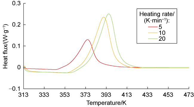
Fig. 1. Heat flux curves at different heating rates. |
Table 1. Phase-transition parameters at different heating rates |
| Heating rates/ (K·min−1) | Onset phase transition temperature | Peak phase transition temperature | Phase transition Heat/(J·g−1) | ||
|---|---|---|---|---|---|
| Celsius temperature/°C | Absolute temperature/K | Celsius temperature/°C | Absolute temperature/K | ||
| 5 | 84.6 | 357.75 | 102.07 | 375.22 | 32.07 |
| 10 | 98.57 | 371.72 | 117.36 | 390.51 | 31.4 |
| 20 | 103.42 | 376.57 | 122.28 | 395.43 | 32.1 |
Based on the DSC experimental results shown in Fig. 1 and Table 1 , the reaction kinetics equation for PF can be established using the Kissinger method, Crane equation, and Malek method [9]:
$ \alpha(t)=1-\left[1-1.8 \times 10^{8} \exp \left(-\frac{8530}{T}\right) t\right]^{12.09}$
According to Eq. (1), the conversion rate of PF at different temperatures and times can be calculated, enabling the determination of the heat released at any given time.
1.2. Fracture temperature field model
As shown in Fig. 2 , a microelement with a length, width, and height of dx, dy, and dz, respectively within the fracture is analyzed. Heat transfer in this microelement involves four components: The fluid within the fracture continuously moves forward, resulting in heat convection. A temperature gradient exists within the fracture, causing heat conduction between adjacent microelements. Heat exchange occurs between the fracturing fluid within the fracture and the surrounding rock mass. PF releases a certain amount of heat during the phase transition process. Therefore, the temperature field of the fluid within the fracture must account for the effects of heat convection, heat conduction, heat exchange, and phase-transition heat release.
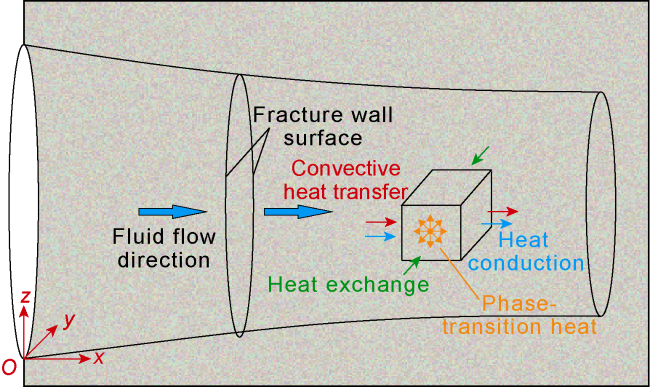
Fig. 2. Physical model of the temperature field within the fracture. |
The fracture temperature field model, which includes factors such as heat convection, heat conduction, heat exchange, and phase-transition heat, is expressed as:
$ \begin{array}{l} \lambda_{\mathrm{w}}\left(\frac{\partial^{2} T_{\mathrm{w}}}{\partial X^{2}}+\frac{\partial^{2} T_{\mathrm{w}}}{\partial y^{2}}+\frac{\partial^{2} T_{\mathrm{w}}}{\partial Z^{2}}\right)- \\ c_{\mathrm{w}} \rho_{\mathrm{w}} \frac{K_{\mathrm{f}}}{\mu}\left(\frac{\partial p}{\partial X} \frac{\partial T_{\mathrm{w}}}{\partial X}+\frac{\partial p}{\partial y} \frac{\partial T_{\mathrm{w}}}{\partial y}+\frac{\partial p}{\partial Z} \frac{\partial T_{\mathrm{w}}}{\partial Z}\right)+ \\ \frac{\lambda_{\mathrm{r}}}{W / 2}\left(T_{\mathrm{r}}-T_{\mathrm{w}}\right)+m_{\mathrm{pf}} \Delta H_{\mathrm{R}} \frac{\mathrm{~d} \alpha}{\mathrm{~d} t} \frac{1}{\mathrm{~d} x \mathrm{~d} y \mathrm{~d} Z}=c_{\mathrm{w}} \rho_{\mathrm{w}} \frac{\partial T_{\mathrm{w}}}{\partial t} \end{array}$
1.3. Rock temperature field model
For the rock temperature field, a physical model of the formation rock temperature field, as shown in Fig. 3 , is established. A microelement with a length, width, and height of dx, dy, and dz, respectively, is analyzed. The heat within this microelement is influenced by heat conduction between adjacent microelements and convective heat transfer of the fluid within the matrix.
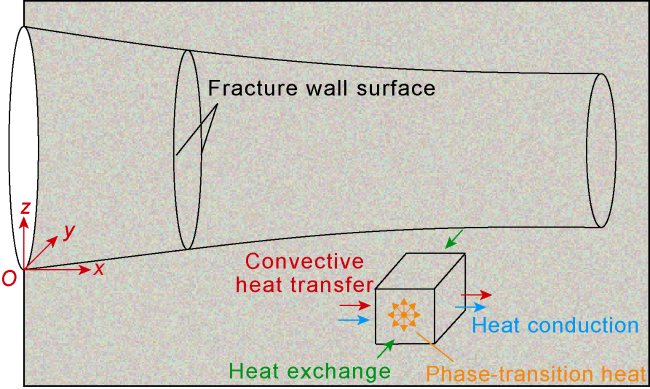
Fig. 3. Physical model of the temperature field in the formation rock mass. |
The establishment of the formation rock temperature field model requires the following assumptions: (1) The thermodynamic parameters of the rock and fracturing fluid are homogeneous and constant. (2) The effects of friction and kinetic energy on heat exchange are negligible. (3) The rock matrix and pore fluid can satisfy local thermal equilibrium conditions. (4) The thermodynamic parameters of the formation are weighted averages of the rock skeleton and pore fluid. Under these assumptions, the temperature field model for the formation rock is expressed as:
$ \begin{array}{l} \lambda_{x} \frac{\partial}{\partial X}\left(\frac{\partial T_{\mathrm{r}}}{\partial X}\right)+\lambda_{y} \frac{\partial}{\partial y}\left(\frac{\partial T_{\mathrm{r}}}{\partial y}\right)+\lambda_{z} \frac{\partial}{\partial z}\left(\frac{\partial T_{\mathrm{r}}}{\partial z}\right)- \\ c_{\mathrm{mw}} \rho_{\mathrm{mw}} \phi\left(V_{x} \frac{\partial T_{\mathrm{r}}}{\partial x}+V_{y} \frac{\partial T_{\mathrm{r}}}{\partial y}+V_{z} \frac{\partial T_{\mathrm{r}}}{\partial z}\right)+ \\ m_{\mathrm{pm}} \Delta H_{\mathrm{R}} \frac{\mathrm{~d} \alpha}{\mathrm{~d} t} \frac{1}{\mathrm{~d} x \mathrm{~d} y \mathrm{~d} z}=c_{\mathrm{r}} \rho_{\mathrm{r}} \frac{\partial T_{\mathrm{r}}}{\partial t} \end{array}$
2. Model solution and validation
2.1. Solution method
At the initial time, the temperature throughout the entire physical model is equal to the original reservoir temperature, expressed as:
$ T_{r}(x, y, z, t)=T_{r e s}(t=0)$
The boundary conditions are:
$ \left\{\begin{array}{ll} q(x, t)=q_{\mathrm{in}} \forall t_{\mathrm{i}} x=0 \\ J_{r}(x, t)=J_{\mathrm{ff}} \forall t_{\mathrm{f}} x=0 \\ J_{r}(x, y, z, t)=J_{\mathrm{res}} \forall x, \forall z, \forall t_{\mathrm{t}} y \rightarrow Y_{\mathrm{max}} \\ J_{\mathrm{m}}=J_{\mathrm{b}} \quad 0<x<L_{\mathrm{f}}, y=w / 2,-H_{\mathrm{f}} / 2<z<H_{\mathrm{f}} / 2 \end{array}\right.$
In Eq. (5), the first expression indicates that the injection velocity at the fracture mouth is constant at any time and equals qin. The second expression states that the fracture mouth temperature at any time equals the bottom hole temperature Twf, which is calculated using the wellbore temperature field model [5]. The third expression specifies that the temperature at the outer boundary of the physical model equals the original reservoir temperature Tres. The fourth expression states that the fluid temperature Tw at the inner side of the fracture wall equals the matrix rock temperature Tb at the outer side of the fracture wall.
The finite element method was employed to solve the temperature fields of the fracture and the formation rock mass. The solution domain was discretized into elements, with the matrix rock represented by four-node tetrahedral elements and the fracture by triangular elements. The temperature field of the fracture element, Tw,e, is expressed as an interpolation of the nodal temperatures [10], as follows:
$ T_{\boldsymbol{w}, \mathrm{e}}(x, y, z)=\boldsymbol{N}(x, y, z) \boldsymbol{q}_{\mathrm{T}, \mathrm{e}}$
The calculation formula for the shape function matrix is given as [11]:
$ N_{i}=\frac{1}{6 V}\left(a_{i}+b_{i} y+c_{y} y+d_{i} z\right)$
Using the Galerkin method [12], the fracture temperature field in Eq. (2) is discretized as:
$ R T_{\pi}+S \frac{\partial T_{\pi}}{\partial t}=\boldsymbol{F}$
The elements of matrices R, S and F are assembled from the corresponding elements of the unit matrices, which are expressed as:
$ \begin{aligned} R_{\mathrm{e}, i j}= & \int_{\Omega_{\mathrm{e}}} \lambda_{\mathrm{w}}\left(\frac{\partial N_{i}}{\partial X} \frac{\partial N_{j}}{\partial x}+\frac{\partial N_{i}}{\partial y} \frac{\partial N_{j}}{\partial y}+\frac{\partial N_{i}}{\partial z} \frac{\partial N_{j}}{\partial Z}\right) \mathrm{d} \Omega+ \\ & \int_{\Omega_{\mathrm{e}}} c_{\mathrm{w}} \rho_{\mathrm{w}} K_{\mathrm{f}} N_{j}\left(\frac{\partial N_{i}}{\partial X} \frac{\partial p}{\partial X}+\frac{\partial N_{i}}{\partial y} \frac{\partial p}{\partial y}+\frac{\partial N_{i}}{\partial z} \frac{\partial p}{\partial Z}\right) \mathrm{d} \Omega \end{aligned}$
$ S_{\mathrm{e}, i, j}=\int_{\Omega} c_{\pi} \rho_{\pi} N_{\mathcal{F}} N \mathrm{~d} \Omega$
$ F_{\mathrm{e}, i}=\int_{\Omega} N_{i}\left[\frac{\lambda_{\mathrm{r}}}{\delta}\left(T_{\mathrm{r}}-T_{\mathrm{w}}\right)+m_{\mathrm{pr}} \Delta H_{\mathrm{R}} \frac{\mathrm{~d} \alpha}{\mathrm{~d} t} \frac{1}{\mathrm{~d} x \mathrm{~d} y \mathrm{~d} z}\right] \mathrm{d} \Omega$
In Eq. (8), the purpose of the time derivative is to determine the unknown Tw,n+1 at time tn+1 based on the known Tw,n at time tn. Since Tw,n is known at tn, and F is also known within the short time step Δt, Eq. (8) can be processed to yield:
$ \begin{array}{l} {\left[\frac{2 S\left(T_{\mathrm{w}, n+1}, t_{n+1}\right)}{\Delta t}+\boldsymbol{R}\left(T_{\mathrm{w}, n+1}, t_{n+1}\right)\right] T_{\mathrm{w}, n+1}=} \\ S\left(T_{\mathrm{w}, n+1}, t_{n+1}\right)\left(\frac{2}{\Delta t} T_{\mathrm{w}, n}+\frac{T_{\mathrm{w}, n+1}-T_{\mathrm{w}, n}}{\Delta t}\right)+F_{n+1} \end{array}$
By applying the same method to discretize Eq. (3), the result is:
$ G T_{r}+H \frac{\partial T_{r}}{\partial t}=E$
Processing Eq. (13) further gives:
$ \begin{array}{l} {\left[\frac{2 H\left(T_{\mathrm{r}, n+1}, t_{n+1}\right)}{\Delta t}+\boldsymbol{G}\left(\boldsymbol{T}_{\mathrm{r}, n+1}, t_{n+1}\right)\right] \boldsymbol{T}_{\mathrm{r}, n+1}=} \\ H\left(\boldsymbol{T}_{\mathrm{r}, n+1}, t_{n+1}\right)\left(\frac{2}{\Delta t} \boldsymbol{T}_{\mathrm{r}, n}+\frac{T_{\mathrm{r}, n+1}-T_{\mathrm{r}, n}}{\Delta t}\right)+E_{n+1} \end{array}$
In Eq. (2), the fluid pressure within the fracture is obtained by solving the Navier-Stokes (N-S) equation [13]. In Eq. (3), the seepage velocities vx, vy, and vz in different directions are determined by solving the fracturing fluid seepage pressure field equation [14]. At each time step, the fracture geometry is calculated by solving the effective stress equilibrium equation [15]. The solution process is shown in Fig. 4.
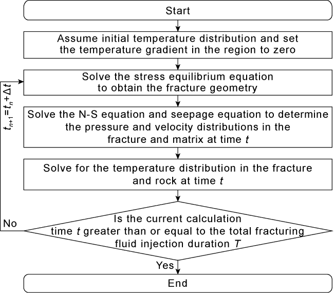
Fig. 4. Solution flowchart for temperature distribution in the fracture and rock mass. |
2.2. Model validation
Using the data listed in Table 2 , the model established in this study was compared with a previously developed fracture temperature field model [16] for validation. In the calculations, the fracture front temperature for both models is equal to the original reservoir temperature, and the temperature at the fracture mouth is approximately the bottom hole temperature. The fracture temperature model established in this study is a three-dimensional model that considers the effects of fluid leak-off and two-dimensional fluid flow within the fracture on the temperature field. As a result, the temperature distribution on any cross-section perpendicular to the fracture length direction exhibits an arch-like shape (Fig. 5a ). In contrast, the model from the literature is a one-dimensional temperature field model, which assumes that the fracturing fluid flows one-dimensionally within the fracture [16]. Consequently, the temperature is uniform across any cross-section perpendicular to the fracture length direction (Fig. 5b ).
Table 2. Main parameters for temperature field calculation |
| Parameter | Value | Parameter | Value |
|---|---|---|---|
| Injection rate | 6 m3/min | Injection time | 60 min |
| Reservoir thickness | 40 m | Porosity | 20% |
| Surface temperature | 20 °C | Reservoir temperature | 110 °C |
| PFFS thermal conductivity | 0.165 W/(m·K) | PFFS specific heat capacity | 2 200 J/(kg·K) |
| Rock thermal conductivity | 3 W/(m·K) | PF volume fraction | 0.3 |
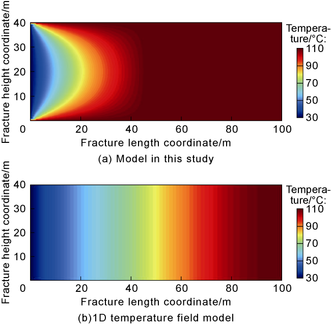
Fig. 5. Temperature distribution in the fracture calculated by two methods (as per the coordinate system in |
Since the model in this study uses four-node tetrahedral elements for the matrix rock and triangular elements for the fracture, it is challenging for element nodes to precisely align with the central axis of the fracture. In contrast, the one-dimensional temperature field model employs a difference method, with element edges perpendicular to each other, allowing all element nodes to be distributed along the central axis. Consequently, when extracting temperature values along the fracture central axis in this model, the coordinates in the fracture height direction may slightly deviate from the axis, resulting in a less smooth temperature curve compared with the one-dimensional model. Reducing the element size can improve the smoothness of the temperature curve. However, considering the significant computational load of the three-dimensional model, this study is seeking a balance between improving curve smoothness and reducing computational workload. An appropriate element size was chosen while ensuring computational accuracy. A comparison of the temperature distributions along the fracture central axis from the two models shows some differences (Fig. 6 ), but the differences are minor, indicating that the model presented in this study has high reliability.
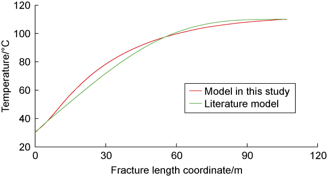
Fig. 6. Comparison of calculation results between the model in this study and the one-dimensional model. |
3. Model application and case analysis
Using the parameters listed in Table 2 , the fracture temperature field under different conditions was calculated to analyze the influence of various factors on the temperature field.
3.1. Effect of phase-transition heat on fracture temperature
Phase-transition heat refers to the amount of heat released by PF per unit mass (Table 1 ). The phase-transition heat values measured under heating rates of 5, 10, and 20 K/min are 32.07, 31.40, and 32.10 J/g, respectively, with an average value of 31.86 J/g. To analyze the influence of phase-transition heat on the fracture temperature field, the temperature distributions under phase-transition heat values of 0, 20, 40, and 60 J/g were calculated (Fig. 7 ). The results indicate that the larger the phase-transition heat, the higher the relative temperature within the fracture. Furthermore, the temperature difference near the fracture mouth is significant under different phase- transition heat conditions, while the temperature difference decreases as the distance to the fracture tip increases. At injection times of 5, 20, 40, and 60 min, the maximum temperature difference occurs at approximately 0, 7, 10, and 10 m from the fracture mouth along the central axis under different phase-transition heat conditions. This phenomenon can be attributed to the following reasons: (1) At an injection time of 5 minutes, the overall temperature within the fracture is relatively high. PF undergoes substantial phase transition near the fracture mouth, and the resulting phase-transition heat significantly raises the temperature at the mouth (Fig. 7a ). (2) At an injection time of 20 min, the temperature at the fracture mouth is lower, and the temperature gradually increases along the fracture length. The temperature at the mouth is below the critical phase-transition temperature of PF, resulting in a lower phase transition rate and limited temperature increase at the mouth. However, at approximately 7 m within the fracture, the temperature rises to the critical value for substantial PF phase transition, causing a significant temperature increase due to the release of phase-transition heat. Beyond 7 m, the remaining PF and phase-transition volume decrease, leading to a reduced temperature variation caused by phase-transition heat (Fig. 7b ). Sustained injection of low- temperature fracturing fluid does not cause an indefinite temperature drop but rather leads to a gradual stabilization [17]. (3) At injection times of 40 and 60 min, the temperature differences within the fracture under different phase-transition heat conditions are minimal. The temperature at the fracture mouth remains low, with limited PF undergoing phase transition, resulting in a small temperature rise. At approximately 10 m within the fracture, the temperature rises sufficiently to trigger substantial PF phase transition. Beyond 10 m, the remaining PF and phase-transition volume are minimal, reducing the temperature variation caused by phase-transition heat (Fig. 7c and 7d).
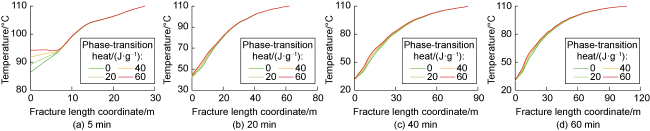
Fig. 7. Temperature along the central axis in the fracture length direction at different injection times. |
To validate the above conclusions, the PF phase transition conversion rates at different times were derived for a phase-transition heat of 40 J/g (Fig. 8 ). These values represent the absolute conversion rate of PF at each grid cell, calculated directly using Eq. (1). Additionally, the rate of change of PF conversion rates at different times for a phase-transition heat of 40 J/g was determined (Fig. 9 ). This value is the total conversion rate difference between two adjacent grid cells in the length direction in Fig. 8 . Fig. 8 shows that at injection times of 5, 20, 40, and 60 min, the PF conversion rates along the central axis within the fracture reach approximately 1.0 at distances of about 15, 40, 48 and 52 m from the fracture mouth, respectively. The lower the temperature along the fracture central axis, the farther the 1.0 conversion rate isoline is from the fracture mouth. The rate of change of PF conversion rates in Fig. 9 reflects the total volume of PF undergoing phase transition at a specific location, as well as the heat released and the magnitude of the temperature increase at that location. From the perspective of the rate of change of conversion rate, the maximum rate of change of conversion rate along the central axis within the fracture occurs at distances of approximately 0, 7, 10, and 10 m from the fracture mouth for injection times of 5, 20, 40 and 60 min, respectively. Therefore, the largest temperature increases occur at these positions, validating the temperature calculation results shown in Fig. 7.
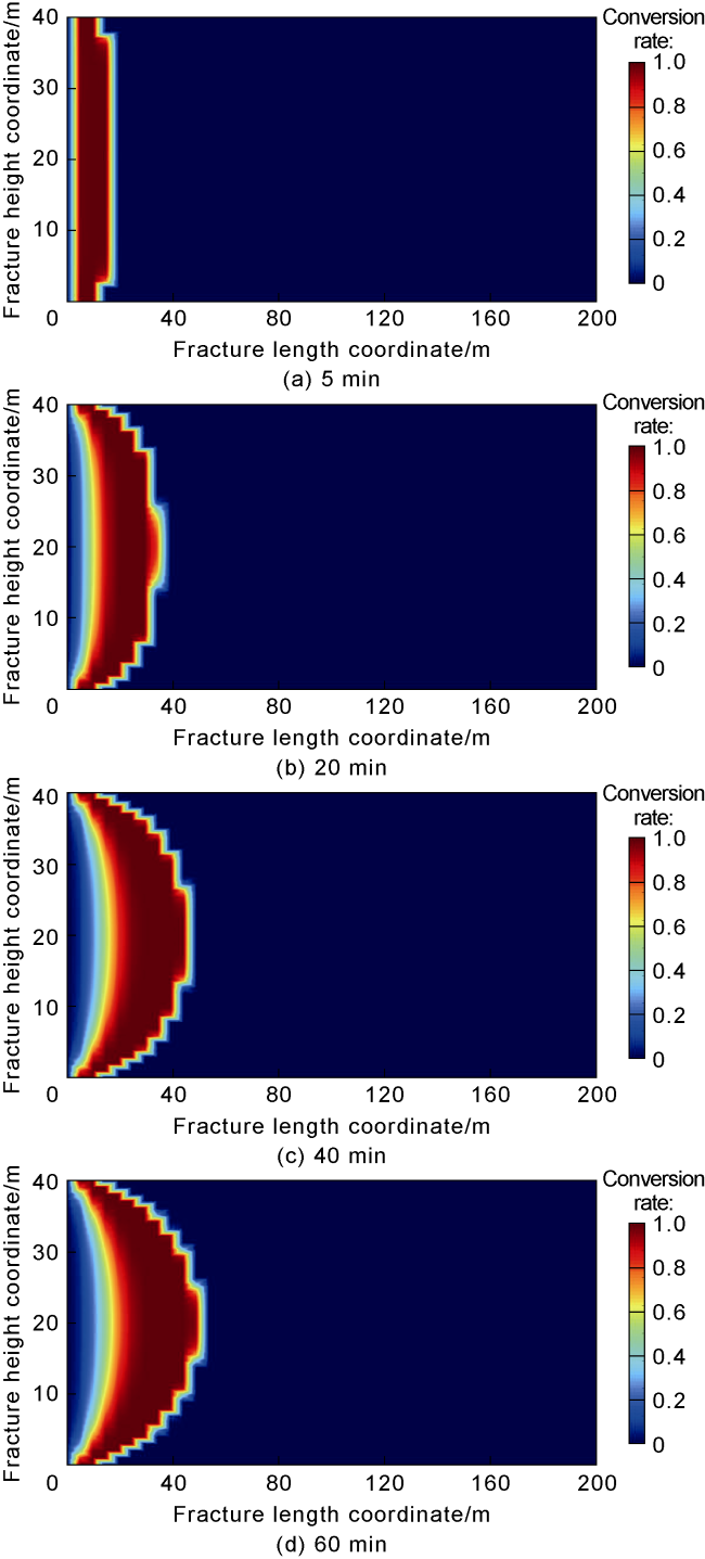
Fig. 8. PF phase transition conversion rates at different injection times for a phase-transition heat of 40 J/g. |
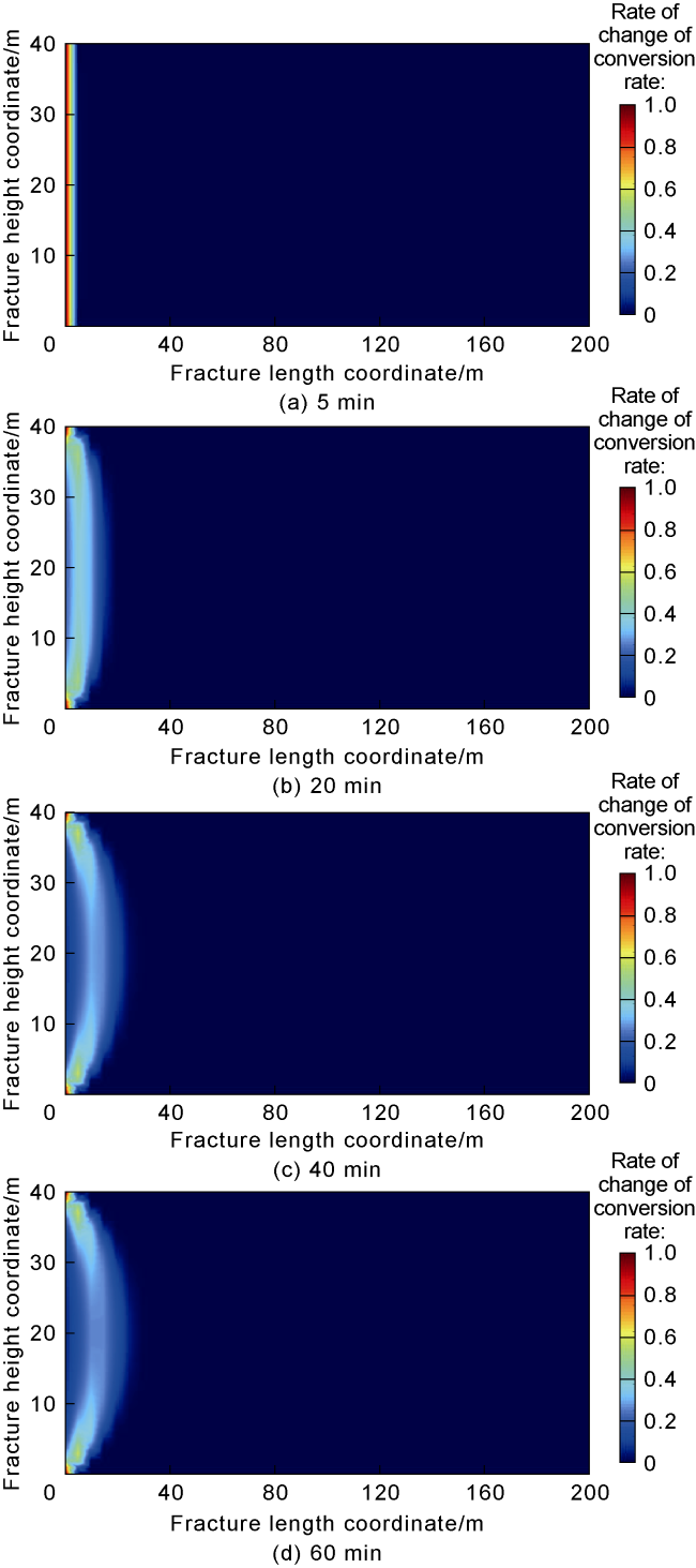
Fig. 9. Rate of change of PF conversion rates at different injection times for a phase-transition heat of 40 J/g. |
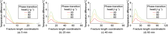
Fig. 10. Temperature difference curves with and without considering phase-transition heat. |
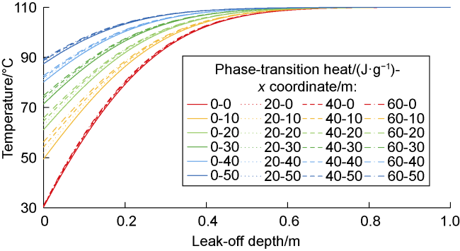
Fig. 11. Temperature distribution in the fracture leak-off direction under different phase-transition heat conditions. |
3.2. Effect of PF volume fraction on fracture temperature
PF and NPF jointly form the PFFS. During field fracturing operations, PF and NPF are injected into the wellbore through separate pipelines. For different reservoirs, the volume fractions of PF and NPF are not equal[18]. To investigate the impact of PF volume fraction on the fracture temperature field, PF volume fractions were set at 10%, 20%, 30% and 40%, respectively based on the data in Table 2 , to analyze their effects on the temperature along the fracture central axis (Fig. 12 ). As shown in the figure, the higher the PF volume fraction, the greater the heat released during PF phase transition, resulting in a larger temperature increase within the fracture. At an injection time of 5 min, the effect of PF volume fraction on the temperature difference is mainly observed at the fracture mouth. When the PF volume fractions are 10%, 20%, 30% and 40%, the temperatures at the fracture mouth are 88.1, 89.9, 91.7 and 93.5 °C, respectively. At injection times of 20, 40 and 60 min, the temperature differences primarily appear near the fracture mouth. At the far end of the fracture, the temperature within the fracture equals the original reservoir temperature.
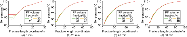
Fig. 12. Temperature along the fracture central axis under different PF volume fraction conditions. |
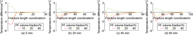
Fig. 13. Temperature difference curves between PF volume fractions of 10%, 20%, 40% and 30% along the fracture. |
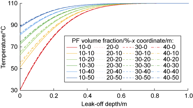
Fig. 14. Temperature distribution in the leak-off direction under different PF volume fraction conditions. |
3.3. Effect of specific heat capacity on fracture temperature
The specific heat capacity of PFFS determines the magnitude of temperature change for a given heat change. Based on the data in Table 2 , the PFFS specific heat capacity was set to 1 700, 2 200, 2 700 and 3 200 J/(kg·K), with the baseline value being 2 200 J/(kg·K) as shown in Table 2 . The influence of specific heat capacity on the fracture temperature field was analyzed (Fig. 15 ). As shown in the figure, when the low-temperature PFFS is injected into the formation, it absorbs heat from the formation, raising its temperature, while the phase transition of PFFS releases heat, further increasing the temperature. Therefore, the smaller the specific heat capacity, the higher the temperature within the fracture. At an injection time of 5 min, the temperatures at the fracture mouth for specific heat capacities of 1 700, 2 200, 2 700 and 3 200 J/(kg·K) are 93.4, 91.8, 90.8 and 90.1 °C, respectively. As the injection time increases, the fracture mouth temperature gradually decreases.
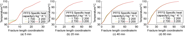
Fig. 15. Temperature variation along the fracture central axis under different specific heat capacities. |
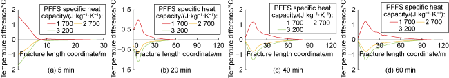
By defining a specific heat capacity of 2 200 J/(kg·K) as the baseline, the fracture central axis temperatures under specific heat capacities of 1 700, 2 700 and 3 200 J/(kg·K) were compared with those under the baseline condition (Fig. 16 ). Since the temperature of the injected fracturing fluid is lower than the original reservoir temperature, the fracturing fluid absorbs heat from the reservoir rock and releases heat during the phase transition, leading to a temperature increase. The larger the specific heat capacity, the smaller the magnitude of the temperature increase. As a result, when the specific heat capacity is 1700 J/(kg·K), the temperature of the fracturing fluid along the fracture central axis is higher than that under the baseline condition, and the temperature difference is positive. Conversely, when the specific heat capacities are 2 700 and 3 200 J/(kg·K), the temperature of the fracturing fluid along the fracture central axis is lower than that under the baseline condition, and the temperature difference is negative.
Fig. 16. Temperature difference curves between fracturing fluid temperatures along the fracture central axis under different specific heat capacities and that under the baseline condition. |
4. Conclusions
The impact of phase-transition heat on fracture temperature is significant and cannot be ignored. The phase- transition process is primarily temperature-controlled, and accurately predicting fracture temperature is crucial for the success of self-propping phase-transition fracturing. Compared with the temperatures without considering phase-transition heat, when the phase-transition heat is 20, 40 and 60 J/g, the maximum temperature increases at the end of fluid injection are 2.1, 4.2 and 6.2 °C, respectively. Phase-transition heat and PF volume fraction are positively correlated with fracture temperature changes, while specific heat capacity is negatively correlated with temperature changes.
At different positions within the fracture and different times, the temperature is alternately dominated by the cooling effect of the injected low-temperature fluid and the heat release during the PF phase-transition process. During the initial stage of fracturing fluid injection, the fracture temperature is higher, and the phase transition is faster, resulting in a significant impact of phase-transition heat on reservoir rock temperature. In the later stage of injection, the fracture temperature decreases, the phase-transition heat release slows, and the cooling effect of the fracturing fluid on the reservoir rock becomes more pronounced. At injection times of 40 and 60 min, the maximum phase-transition rate and the maximum temperature difference occur approximately 10 m from the fracture mouth.
Nomenclature
a, b, c, d—coefficients related to the geometric positions of nodes, dimensionless;
cmw—specific heat capacity of fluid in the matrix, J/(kg·K);
cr—specific heat capacity of rock, J/(kg·K);
cw—specific heat capacity of fracturing fluid in the fracture, J/(kg·K);
E—temperature load vector of the rock temperature field;
F—temperature load vector of the fracture temperature field;
Fe,i—element of the temperature load vector for unit fracture temperature field;
G—thermal conductivity matrix of the rock temperature field;
Hf—fracture height, m;
H—heat capacity matrix of the rock temperature field;
ΔHR—heat released during PF curing reaction, J/kg;
i, j—serial number;
Kf—fracture permeability, m2;
Lf—fracture length, m;
mpf—mass of PF contained in a hexahedral fracture microelement, kg;
mpm—mass of PF contained in a hexahedral rock microelement, kg;
n—time step;
Ni—element of matrix N;
N(x,y,z)—interpolation matrix;
p—fluid pressure within the fracture, Pa;
q—boundary injection rate, m3/min;
qin—constant injection rate, m3/min;
qT,e—node temperature matrix, K;
R—thermal conductivity matrix of the fracture temperature field;
Re,i,j—element of the thermal conductivity matrix for the fracture temperature field;
S—heat capacity matrix of the fracture temperature field;
Se,i,j—element of the heat capacity matrix for the fracture temperature field;
t—time, s;
T—temperature, K;
Tb—boundary temperature, K;
Tr—rock temperature, K;
Tres—original reservoir temperature, K;
Tr—matrix of the rock temperature field;
Tw—temperature on the inner side of the fracture wall surface, K;
Tw—temperature matrix of the fracture temperature field;
Tw,e—temperature of a fracture element, K;
Twf—bottom hole temperature, K;
vx, vy, vz—seepage velocities in different coordinate directions, m/s;
V—volume of the element, m3;
w—fracture width, m;
x, y, z—cartesian coordinates, m;
ymax—position at infinity in the fracture width direction, m;
α—conversion rate, dimensionless;
$ \alpha(t)$—conversion rate at time t, dimensionless;
δ—fracture half-width, m;
λr—heat transfer coefficient between fracturing fluid and rock, W/(m2·K);
λx, λy, λz—thermal conductivity of rock in different coordinate directions, W/(m·K);
λw—thermal conductivity, W/(m·K);
μ—viscosity of fluid in the fracture, Pa•s;
ρmw—density of fluid in the matrix, kg/m3;
ρr—density of rock, kg/m3;
ρw—density of fracturing fluid, kg/m3;
ϕ—Porosity of matrix rock, dimensionless;
Ω—integral domain;
Ωe—element integral domain.