

Introduction
The extraction of liquid or gas from reservoirs alters the stress and deformation fields in surrounding rocks, leading to reservoir compaction, which is called reservoir development induced deformation. Rock deformation significantly affects production capacity but may also trigger reservoir damage and subsidence hazards [1-2]. Numerous scholars have conducted research through theoretical analyses, laboratory experiments, and field observations. Specifically, the model of deformation induced by reservoir development, as a core component of the fluid flow-geomechanics coupling theoretical framework for reservoirs [3-5], quantitatively characterizes the mechanism of pore pressure changes on deformation fields, playing a critical role in efficient reservoir development.
The theoretical foundation for fluid injection and production induced deformation was initiated by Terzaghi’s mathematical model for soil consolidation [6], followed by Biot’s classical three-dimensional consolidation theory [7], which laid the groundwork for modern fluid flow-geomechanics coupling studies. However, Biot’s theory did not explicitly define flow and deformation boundary conditions. In 1957, Geertsma [8] introduced assumptions of constant overburden pressure and uniaxial deformation during reservoir production, refining Biot’s theory for reservoir development applications. In 1973, Geertsma [9] further integrated Mindlin’s influence functions [10] and established the analytical solution for surface displacement in reservoirs with uniform pressure depletion through boundary integration. However, this approach remained limited by idealized geometric configurations and elastic medium assumptions. To overcome the limitations of analytical methods under complex geological conditions, numerical simulation gradually became the mainstream approach. Morita et al. [11] derived finite element models for total and effective stresses in reservoirs under constant pressure depletion. Subsequent studies adopted iterative coupling between mechanical solvers (e.g., Abaqus [12-13], FLAC3D [14]) and reservoir simulators (e.g., Eclipse), while also developing fully coupled finite element models [15-16]. Since the 21st century, unconventional reservoir development has driven research toward complex fractured reservoirs. Scholars have explored models such as equivalent continuum [17], discrete fractures [18-20], and embedded discrete fractures [21-23], evolving various innovative algorithms including the boundary element method (BEM)[24-25], extended finite element method (XFEM) [26-28], finite volume method (FVM) [29], discontinuous Galerkin method [30], and mixed finite element methods [31-32]. Although these methods have advanced the precise characterization of local mechanical fields in fractures, they retain traditional approaches for reservoir deformation boundaries: defining the reservoir domain as the flow-deformation calculation region while simplifying external strata as constant stress or displacement conditions at reservoir boundaries [33-34], or extending the deformation calculation domain outward from reservoir edges with assigned boundary conditions. However, development-induced deformation is inherently linked to semi-infinite strata. Such boundary simplifications introduce computational inaccuracies. Studies by Wu et al. [35] demonstrated that the size of the deformation calculation domain significantly affects results. Consequently, mainstream commercial software typically extends the deformation calculation domain but uses large external grids to maintain computational feasibility [36].
The current finite element-based methods for development-induced deformation suffer from three major limitations: incomplete consideration of semi-infinite strata, inadequate treatment of flow boundaries’ influence on deformation, and low accuracy in far-field deformation due to oversized external grids [37]. To address these issues, this study proposes a novel equivalent force model for reservoir development-induced deformation from a semi-infinite strata perspective, through detailed mechanical analysis to reveal the mechanisms by which internal reservoir flow and flow boundaries govern deformation. Furthermore, a volumetric boundary element method is developed to achieve precise full-space-domain calculations. This approach establishes a foundation for accurate and efficient numerical simulation of fluid flow-geomechanics coupling in reservoir development.
1. Fundamental equations
Consider an arbitrary infinitesimal element within the strata, whose volume is sufficiently large relative to the pore structure yet sufficiently small compared to the entire strata. This element is treated as a homogeneous material. Throughout the analysis, it is critical to ensure that the properties of the element remain consistent with those in the actual strata. For example, the pores and rock skeleton on the element’s surface do not act simultaneously on a closed boundary (except for separately discussed closed boundary surfaces). Instead, the pores connect to pores outside the element, and the rock skeleton connects to the rock skeleton outside the element, with the two systems being independently linked.
Stress is defined as the internal force acting per unit area, representing the intensity of internal force distribution. Therefore, the definition of stress must specify the corresponding area. In this study, the area corresponding to rock skeleton stress is defined as the apparent area of the rock, rather than the actual skeleton area. The actual skeleton stress corresponds to the skeleton area, the relationship between the rock skeleton stress and the actual skeleton stress is expressed as:
$ \sigma_{i j}=(1-\phi) \sigma_{s, i j} \cdot(i=x, \cdot y, \cdot z ; j=x, \cdot y, z) $
Based on this definition, the total stress on any cross- section within the rock is [38]:
$ \sigma_{\mathrm{t}, i j}=\sigma_{i j}-\phi p \delta_{i j}$
In Eq. (2), the pore fluid pressure is a compressive stress, so the fluid stress is expressed as −p.
The equilibrium equation for the rock skeleton is [39]:
$ \frac{\partial \sigma_{i j}}{\partial x_{j}}+f_{i}=0$
The geometric equation for the rock skeleton is [39]:
$ \varepsilon_{i j}=\frac{1}{2}\left(\frac{\partial u_{i}}{\partial x_{j}}+\frac{\partial u_{j}}{\partial x_{i}}\right)$
The constitutive equation for an isotropic, linearly elastic, porous medium is [39]:
$ \sigma_{\mathrm{t}, i j}=2 G \varepsilon_{i j}+\frac{2 G v}{1-2 v} \delta_{i j} \varepsilon-\left(1-\frac{K_{\mathrm{p}}}{K_{\mathrm{s}}}\right) \delta_{i j} p$
where $ \mathcal{E}=\varepsilon_{x x}+\varepsilon_{y y}+\varepsilon_{z z}$
By substituting Eq. (2) into Eq. (5), Eq. (6) can be acquired:
$ \sigma_{i j}=2 G \varepsilon_{i j}+\frac{2 G v}{1-2 v} \delta_{i j} \varepsilon-\left(1-\phi-\frac{K_{\mathrm{p}}}{K_{\mathrm{s}}}\right) \delta_{i j} p$
2. Equivalent force model of deformation induced by reservoir development
2.1. Flow equivalent force
When subsurface fluid injection and production induce changes in reservoir pore pressure, the stress within the rock skeleton simultaneously changes. Due to the extremely low flow velocity of fluid through rock pore throats, the fluid can be considered quasi-static, i.e., in a state of mechanical equilibrium. Similarly, the rock skeleton also remains in a quasi-static state of mechanical equilibrium. The state of force interaction between the fluid and the skeleton is depicted in Fig. 1.
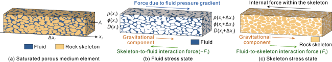
Fig. 1. Force analysis of strata elements. |
Based on Fig. 1b , the equation for fluid force equilibrium can be established:
$ \begin{array}{c} A\left[\left.(p \phi)\right|_{x_{i}}-\left.(p \phi)\right|_{x_{i}+\Delta x_{i}}\right]+\rho_{\mathrm{f}} g A \Delta x x_{i} \phi \frac{\left.D\right|_{x_{i}+\Delta x_{i}}-\left.D\right|_{x_{i}}}{\Delta x_{i}}-. \\ F_{i} A \Delta x_{i}=0 \end{array}$
Dividing both sides of Eq. (7) by AΔxi and taking the limit as Δxi→0, the volumetric force exerted by the fluid on the skeleton is obtained:
$ F_{i}=-\frac{\partial p \phi}{\partial x_{i}}+\rho_{\mathrm{f}} g \phi \frac{\partial D}{\partial x_{i}}$
Similarly, from Fig. 1c , the total external force experienced per unit apparent volume of the rock skeleton is derived as:
$ f_{i}=F_{i}+\rho_{s} g(1-\phi) \frac{\partial D}{\partial x_{i}}$
By substituting Eq. (8) into Eq. (9), Eq. (10) can be acquired:
$ f_{i}=-\frac{\partial p \phi}{\partial x_{i}}+\bar{\rho} g \frac{\partial D}{\partial x_{i}}$
where $ \bar{\rho}=\rho_{\mathrm{f}} \phi+\rho_{\mathrm{s}}(1-\phi)$
By substituting Eq. (10) into Eq. (3), the equilibrium equation for rock skeleton stress is obtained:
$ \frac{\partial \sigma_{i j}}{\partial x_{j}}-\frac{\partial p \phi}{\partial x_{i}}+\frac{\partial D}{\partial x_{i}} \bar{\rho} g=0$
By substituting Eqs. (4) and (6) into Eq. (11), the differential equation set for skeleton deformation expressed in terms of displacement is achieved:
$ G u_{i, i j}+\frac{G}{1-2 v} u_{j, i j}-\left(1-\frac{K_{\mathrm{p}}}{K_{\mathrm{s}}}\right) \frac{\partial p}{\partial x_{i}}+\frac{\partial D}{\partial x_{i}} \bar{\rho} g=0$
Eq. (12) exhibits complete formal consistency with the Lame-Navier equation (Eq. (13)) derived through the displacement method in elasticity theory [40].
$ G u_{i, j j}+\frac{G}{1-2 v} u_{j i j j}+f_{e, i}=0$
where fe,i represents the flow equivalent force in the i-direction, which can be expressed as:
$ f_{\mathrm{e}, i}=-\left(1-\frac{K_{\mathrm{p}}}{K_{\mathrm{s}}}\right) \frac{\partial p}{\partial x_{i}}+\frac{\partial D}{\partial x_{i}} \bar{\rho} g$
This demonstrates that the deformation of the porous medium skeleton induced by fluid flow is equivalent to general elastic deformation under the action of the flow equivalent force defined in Eq. (14), where this flow equivalent force is a body force.
In oil and gas reservoir development, the primary focus lies on quantifying changes in rock deformation. The increment of the flow equivalent force relative to the initial state is:
$ \Delta f_{\mathrm{e}, i}=-\left(1-\frac{K_{\mathrm{p}}}{K_{\mathrm{s}}}\right) \frac{\partial \Delta p}{\partial x_{i}}+\frac{\partial D}{\partial x_{i}} \Delta \bar{\rho} g\left(x_{i} \in \Omega\right)$
During subsurface fluid injection and production, the fluid density varies significantly with pore pressure and fluid composition, while the mass of the rock skeleton within any element remains virtually constant. Therefore, neglecting $ \Delta\left\lceil\rho_{\mathrm{s}}(1-\phi)\right\rceil$, Eq. (15) can be simplified as:
$ \Delta f_{\mathrm{e}, i}=-\left(1-\frac{K_{\mathrm{p}}}{K_{\mathrm{s}}}\right) \frac{\partial \Delta p}{\partial x_{i}}+\frac{\partial D}{\partial x_{i}} \Delta \rho_{\mathrm{f}} g \phi \cdots\left(\mathrm{x}_{i} \in \Omega\right)$
2.2. Boundary equivalent force
The boundary conditions for deformation induced by reservoir development encompass two types: deformation boundaries of the strata rock and flow boundaries of the fluid. For real strata, complete deformation boundary conditions should include the free boundary at the Earth’s surface and the semi-infinite boundary of the entire crust. Typically, variations in elastic parameters within the reservoir and surrounding strata regions are not significant. To simplify calculations and analysis, this study assumes the strata rock to be a homogeneous elastic material, thereby reducing the problem to an elastic problem of a homogeneous semi-infinite medium with a free surface.
The fluid flow boundary corresponds to the closed boundary of the reservoir, where the normal total stresses on both sides of the closed boundary are balanced (as shown in Fig. 2 ). This can be expressed as:
(xi∈Γ)
where $ n_{\Omega}$ and are the unit inward normal vectors at the closed boundary Γ for the internal and external
domains, respectively, and satisfy . The Einstein summation convention applies to repeated Latin indices in Eqs. (17)-(20).
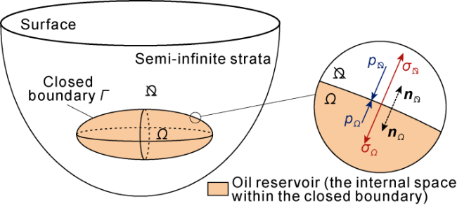
Fig. 2. Mechanical equilibrium across closed boundaries. |
Eq. (17) can be reformulated as:
(xi∈Γ)
By substituting Eqs. (4) and (6) into Eq. (18), Eq. (19) can be acquired:
Eq. (19) exhibits complete formal consistency with the displacement-based continuity condition for normal forces at interfaces in elasticity theory (Eq. (20)) [40]:
where pe,i represents the boundary equivalent force in the i-direction and can be expressed as:
(xi∈Γ)
This demonstrates that the influence of the reservoir’s closed boundary on strata deformation is equivalent to the general elastic deformation induced by applying a boundary equivalent force on the virtual surface of the closed boundary. This boundary equivalent force is a surface force.
The increment of the boundary equivalent force relative to the initial state is:
(xi∈Γ)
No fluid injection and extraction occurs outside the closed boundary of the reservoir, and the pore pressure change outside the closed boundary can be neglected (i.e., ). Therefore, Eq. (22) can be simplified to:
(xi∈Γ)
The above study demonstrates that the effects of internal reservoir flow and flow boundaries on strata deformation can be equivalently represented as the impacts of external forces acting within the reservoir interior and at the reservoir boundaries, respectively. Specifically, the external force equivalent to internal reservoir flow is termed the flow equivalent force, while the external force equivalent to flow boundaries is termed the boundary equivalent force.
2.3. Analytical solution
For real strata, the complete deformation boundary can be regarded as the semi-infinite boundary of the entire crust. Building on the preceding analysis, the strata deformation induced by reservoir development is equivalent to general elastic deformation of a semi-infinite medium under the action of the flow equivalent force within the reservoir interior and the boundary equivalent force at the closed boundaries of the reservoir. Consequently, for the semi-infinite deformation boundaries, by adopting Mindlin’s fundamental solution for a concentrated force in a semi-infinite medium [10] as the Green’s function, the internal reservoir flow and flow boundaries are transformed into two external loading conditions on the semi-infinite strata: the flow equivalent force and the boundary equivalent force. According to the superposition principle, the deformation solution at any point in the strata can be expressed as the convolution of the flow equivalent force, boundary equivalent force, and Green’s function.
The coordinate system is established as shown in Fig. 3 , with the z-axis pointing vertically downward. Consider a unit force applied along the z-axis at an arbitrary point (x, y, z). The displacement at any point (α, β, γ) in the semi-infinite medium is given by Eq. (24) [10]. If the unit force is applied along the x-axis, the displacement at any point (α, β, γ) in the semi-infinite medium is expressed by Eq. (25) [10]. Similarly, for a unit force along the y-axis, the displacement at any point (α, β, γ) is provided in Eq. (26) [10].
$\left\{\begin{aligned} \tilde{u}_{Z_{-} x}= & \frac{\alpha-x}{16 \pi G(1-v)}\left[\frac{\gamma-Z}{R_{1}^{3}}+\frac{(3-4 v)(\gamma-Z)}{R_{2}^{3}}-\right. \\ & \left.\frac{4(1-v)(1-2 v)}{R_{2}\left(R_{2}+\gamma+Z\right)}+\frac{6 \gamma Z(\gamma+Z)}{R_{2}^{5}}\right] \\ \tilde{u}_{Z_{-} y}= & \frac{\beta-y}{16 \pi G(1-v)}\left[\frac{\gamma-Z}{R_{1}^{3}}+\frac{(3-4 v)(\gamma-Z)}{R_{2}^{3}}-\right. \\ & \left.\frac{4(1-v)(1-2 v)}{R_{2}\left(R_{2}+\gamma+Z\right)}+\frac{6 \gamma Z(\gamma+Z)}{R_{2}^{5}}\right] \\ \tilde{u}_{Z_{-} Z}= & \frac{1}{16 \pi G(1-v)}\left[\frac{3-4 v}{R_{1}}+\frac{8(1-v)^{2}-(3-4 v)}{R_{2}}+\right. \\ & \left.\frac{(\gamma-Z)^{2}}{R_{1}^{3}}+\frac{(3-4 v)(\gamma+Z)^{2}-2 \gamma Z}{R_{2}^{3}}+\frac{6 \gamma Z(\gamma+Z)^{2}}{R_{2}^{5}}\right] \end{aligned}\right.$
$\left\{\begin{aligned} \tilde{u}_{X_{-} x}= & \frac{1}{16 \pi G(1-v)}\left\{\frac{3-4 v}{R_{1}}+\frac{1}{R_{2}}+\frac{(\alpha-x)^{2}}{R_{1}^{3}}+\frac{(3-4 v)(\alpha-x)^{2}}{R_{2}^{3}}+\right. \\ & \left.\frac{2 \gamma Z}{R_{2}^{3}}\left(1-\frac{3(\alpha-x)^{2}}{R_{2}^{2}}\right)+\frac{4(1-v)(1-2 v)}{R_{2}+\gamma+Z}\left[1-\frac{(\alpha-x)^{2}}{R_{2}\left(R_{2}+\gamma+Z\right)}\right]\right\} \\ \tilde{u}_{X_{-} y}= & \frac{(\alpha-x)(\beta-y)}{16 \pi G(1-v)}\left[\frac{1}{R_{1}^{3}}+\frac{3-4 v}{R_{2}^{3}}-\frac{6 \gamma Z}{R_{2}^{5}}-\frac{4(1-v)(1-2 v)}{R_{2}\left(R_{2}+\gamma+z\right)^{2}}\right] \\ \tilde{u}_{X_{-} z}= & \frac{\alpha-x}{16 \pi G(1-v)}\left[\frac{\gamma-Z}{R_{1}^{3}}+\frac{(3-4 v)(\gamma-z)}{R_{2}^{3}}-\frac{6 \gamma Z(\gamma+z)}{R_{2}^{5}}+\right. \\ & \left.\frac{4(1-v)(1-2 v)}{R_{2}\left(R_{2}+\gamma+z\right)}\right] \end{aligned}\right.$
$\left\{\begin{aligned} \tilde{u}_{y_{-} x}= & \frac{(\alpha-x)(\beta-y)}{16 \pi G(1-v)}\left[\frac{1}{R_{1}^{3}}+\frac{3-4 v}{R_{2}^{3}}-\frac{6 \gamma x}{R_{2}^{5}}-\frac{4(1-v)(1-2 v)}{R_{2}\left(R_{2}+\gamma+z\right)^{2}}\right] \\ \tilde{u}_{y_{-} y}= & \frac{1}{16 \pi G(1-v)}\left\{\frac{3-4 v}{R_{1}}+\frac{1}{R_{2}}+\frac{(\beta-y)^{2}}{R_{1}^{3}}+\right. \\ & \frac{(3-4 v)(\beta-y)^{2}}{R_{2}{ }^{3}}+\frac{2 \gamma Z}{R_{2}{ }^{3}}\left[1-\frac{3(\beta-y)^{2}}{R_{2}{ }^{2}}\right]+ \\ & \left.\frac{4(1-v)(1-2 v)}{R_{2}+\gamma+Z}\left[1-\frac{(\beta-y)^{2}}{R_{2}\left(R_{2}+\gamma+z\right)}\right]\right\} \\ \tilde{u}_{y_{-} z}= & \frac{(\beta-y)}{16 \pi G(1-v)}\left[\frac{\gamma-Z}{R_{1}^{3}}+\frac{(3-4 v)(\gamma-z)}{R_{2}{ }^{3}}-\frac{6 \gamma Z(\gamma+Z)}{R_{2}^{5}}+\right. \\ & \left.\frac{4(1-v)(1-2 v)}{R_{2}\left(R_{2}+\gamma+Z\right)}\right] \end{aligned}\right.$
where
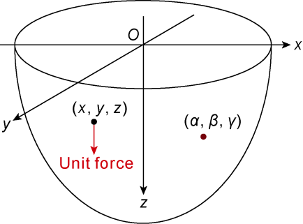
Fig. 3. Semi-infinite medium subjected to a concentrated force. |
The displacement caused by the aforementioned unit forces is defined as the displacement Green’s function $\tilde{u}_{i}(x, y, z, \alpha, \beta, \gamma)$, which represents the displacement component in the j-direction at point (α, β, γ) due to a unit force applied in the i-direction at point (x, y, z).
According to the linear elastic superposition principle, the displacement of the strata induced by reservoir development, relative to the initial state, can be expressed as the convolution of the equivalent force increment and the displacement Green’s function:
$\begin{aligned} \Delta u_{i}(\alpha, \beta, \gamma)= & \iint_{\Gamma}\left(\Delta p_{\mathrm{e}, x} \tilde{u}_{X_{-} i}\right) \mathrm{d} y \mathrm{~d} z+ \\ & \iint_{\Gamma}\left(\Delta p_{\mathrm{e}, y} \tilde{u}_{y_{-} i}\right) \mathrm{d} x \mathrm{~d} z+\iint_{\Gamma}\left(\Delta p_{\mathrm{e}, z} \tilde{u}_{Z_{-} i}\right) \mathrm{d} x \mathrm{~d} y+ \\ & \iiint_{\Omega}\left(\Delta f_{\mathrm{e}, \bar{X}} \tilde{X}_{X_{-} i}+\Delta f_{\mathrm{e}, y} \tilde{u}_{y_{-} i}+\Delta f_{\mathrm{e}, z} \tilde{u}_{Z_{-} i}\right) \mathrm{d} x \mathrm{~d} y \mathrm{~d} z \end{aligned}$
Based on the displacement increment, substituting Eq. (27) into Eq. (4), the apparent strain relative to the initial state can be derived. Subsequently, substituting this strain into Eq. (6) yields the skeleton stress relative to the initial state.
2.4. Volumetric boundary element numerical solution method
The primary challenge in practical reservoir studies lies in irregular reservoir geometries and non-uniform pore pressure changes, which can only be resolved through discrete numerical simulations. Therefore, it is imperative to discretize the aforementioned model.
For the flow equivalent force, the central difference method (with one-sided difference at the reservoir boundary) can be used to discretize Eq. (16) as:
$\left\{\begin{aligned} \Delta f_{\mathrm{e}, z,(a, b, c)}= & -\left(1-\frac{K_{\mathrm{p}}}{K_{\mathrm{s}}}\right) \frac{\Delta p_{(a+1, b, c)}-\Delta p_{(a-1, b, c)}}{2 \Delta x}+ \\ & \frac{D_{(a+1, b, c)}-D_{(a-1, b, c)} \Delta \rho_{\mathrm{f},(a, b, c)} g \phi_{(a, b, c)}}{2 \Delta x} \\ \Delta f_{\mathrm{e}, y,(a, b, c)}= & -\left(1-\frac{K_{\mathrm{p}}}{K_{\mathrm{s}}}\right) \frac{\Delta p_{(a, b+1, c)}-\Delta p_{(a, b-1, c)}}{2 \Delta y}+ \\ & \frac{D_{(a, b+1, c)}-D_{(a, b-1, c)} \Delta \rho_{\mathrm{f}(a, b, c)} g \phi_{(a, b, c)}}{2 \Delta y} \\ \Delta f_{\mathrm{e}, z,(a, b, c)}= & -\left(1-\frac{K_{\mathrm{p}}}{K_{\mathrm{s}}}\right) \frac{\Delta p_{(a, b, c+1)}-\Delta p_{(a, b, c-1)}}{2 \Delta z}+ \\ & \frac{D_{(a, b, c+1)}-D_{(a, b, c-1)} \Delta \rho_{\mathrm{f},(a, b, c)} g \phi_{(a, b, c)}}{2 \Delta z} \end{aligned}\right.$
For the boundary equivalent force, non-boundary grid cells are set to zero, while boundary grid cells are discretized according to Eq. (23):
$\left\{\begin{aligned} \Delta p_{\mathrm{e}, z_{,}(a, b, c)}= & \pm\left(1-K_{\mathrm{p}} / K_{\mathrm{s}}\right) \Delta p_{(a \pm 0.5, b, c)} \\ & {\left[\operatorname{grid}_{(a \pm 1, b, c)} \notin \Omega, \operatorname{grid}_{(a, b, c)} \in \Omega\right] } \\ \Delta p_{\mathrm{e}, y_{,}(a, b, c)}= & \pm\left(1-K_{\mathrm{p}} / K_{\mathrm{s}}\right) \Delta p_{(a, b \pm 0.5, c)} \\ & {\left[\operatorname{grid}_{(a, b \pm 1, c)} \notin \Omega, \operatorname{grid}_{(a, b, c)} \in \Omega\right] } \\ \Delta p_{\mathrm{e}, z,(a, b, c)}= & \pm\left(1-K_{\mathrm{p}} / K_{\mathrm{s}}\right) \Delta p_{(a, b, c \pm 0.5)} \\ & {\left[\operatorname{grid}_{(a, b, c \pm 1)} \notin \Omega, \operatorname{grid}_{(a, b, c)} \in \Omega\right] } \end{aligned}\right.$
For displacement increments, Eq. (27) is discretized as:
$\begin{array}{c} \Delta u_{i}(\alpha, \beta, \gamma)=\sum_{a, b, c}\left[\Delta p_{\mathrm{e}, x,(a, b, c)} \tilde{F}_{x_{-} i}\right]+ \\ \sum_{a, b, c}\left[\Delta p_{\mathrm{e}, y,(a, b, c)} \tilde{F}_{y_{-} i}\right]+\sum_{a, b, c}\left[\Delta p_{\mathrm{e}, Z,(a, b, c)} \tilde{F}_{Z_{-} i}\right]+ \\ \sum_{a, b, c}\left[\Delta f_{\mathrm{e}, X_{,}(a, b, c)} \tilde{V}_{x_{-} i}+\Delta f_{\mathrm{e}, y_{,}(a, b, c)} \tilde{V}_{y_{-} i}+\Delta f_{\mathrm{e}, Z,(a, b, c)} \tilde{V}_{Z_{-} i}\right] \end{array}$
where represents the grid volume source, and $\tilde{F}_{i j}$ represents the grid boundary source:
$\left\{\begin{array}{l} \tilde{V}_{j_{-} i}=\int_{c-0.5}^{c+0.5} \int_{b-0.5}^{b+0.5} \int_{a-0.5}^{a+0.5} \tilde{u}_{j_{-} i} \mathrm{~d} x \mathrm{~d} y \mathrm{~d} z \\ \tilde{F}_{x_{-} i}=\int_{c-0.5}^{c+0.5} \int_{b-0.5}^{b+0.5} \tilde{u}_{x_{-} i} \mathrm{~d} y \mathrm{~d} z \\ \tilde{F}_{y_{-} i}=\int_{c-0.5}^{c+0.5} \int_{a-0.5}^{a+0.5} \tilde{u}_{y_{-} i} \mathrm{~d} x \mathrm{~d} z \\ \tilde{F}_{z_{-} i}=\int_{b-0.5}^{b+0.5} \int_{a-0.5}^{a+0.5} \tilde{u}_{z_{-} i} \mathrm{~d} x \mathrm{~d} y \end{array}\right.$
In Eq. (31), the grid boundary source is derived by surface integration of the Green’s function over reservoir boundary grids, while the grid volume source is obtained by volume integration of the Green’s function over reservoir interior grids. The deformation solution at any strata point is then calculated by multiplying grid boundary equivalent forces with corresponding boundary sources, grid flow equivalent forces with corresponding volume sources, and summing the results (Eq. 30).
The numerical method presented above shares conceptual similarities with the boundary element method (BEM). However, a key distinction lies in the integral equation shown in Eq. (30) of this work. In addition to requiring surface integration over the reservoir’s flow boundaries (where boundary equivalent forces, i.e., surface forces, act), it necessitates volume integration over the reservoir’s interior (where flow equivalent forces, i.e., body forces, exist). Due to this dual integration framework—combining both surface and volume terms—the proposed method is termed the volumetric boundary element method (VBEM).
3. Model validation and testing
Direct deformation estimation using reservoir property fields at specific times and initial states effectively evaluates the accuracy of deformation solvers. This study first validates the analytical solution in Eq. (27) by recovering Geertsma’s method [9], followed by comparative testing with the commercial numerical simulator VISAGE using deformation calculations for a depleted reservoir.
3.1. Analytical solution validation
Geertsma [9] derived an analytical solution for subsidence induced by uniform pressure depletion in a thin, circular reservoir. Reservoir parameters are listed in Table 1 .
Table 1. Reservoir parameters for analytical solution validation |
| Parameter | Value | Parameter | Value |
|---|---|---|---|
| Bulk modulus of the skeleton material | 35 000 MPa | Reservoir thickness | 10 m |
| Apparent bulk modulus | 2 000 MPa | Reservoir top depth | 1 000 m |
| Apparent shear modulus | 1 200 MPa | Reservoir radius | 1 000 m |
| Apparent Poisson’s ratio | 0.25 | Initial pressure | 30 MPa |
| Porosity | 20% | Pressure increment | -10 MPa |
| Fluid density (Reference pressure) | 800 kg/m3 (30 MPa) | Total compressibility | 3×10⁻³ MPa-1 |
The state equation is given by:
$\Delta\left(\rho_{\mathrm{f}} \phi\right)=\rho_{\text {ref }} C_{\mathrm{t}}\left(p-p_{0}\right)$
According to Eq. (16), since the pressure within the reservoir is uniformly distributed, the flow equivalent force can be derived as:
$\left\{\begin{array}{l} \Delta f_{\mathrm{e}, z}=\Delta f_{\mathrm{e}, y}=0 \\ \Delta f_{\mathrm{e}, z}=\Delta\left(\rho_{\mathrm{f}} \phi\right) g \end{array} \quad\left(x^{2}+y^{2} \leq R^{2}, D_{\mathrm{t}} \leq z \leq D_{\mathrm{t}}+h\right)\right.$
According to Eq. (23), the boundary equivalent force at the top of the reservoir is derived as:
$\left\{\begin{array}{l} \Delta p_{\mathrm{e}, z}=\Delta p_{\mathrm{e}, y}=0 \\ \Delta p_{\mathrm{e}, z}=-\left(1-K_{\mathrm{p}} / K_{\mathrm{s}}\right) \Delta p \end{array} \quad\left(x^{2}+y^{2} \leq R^{2}, z=D_{\mathrm{t}}\right)\right.$
Similarly, the boundary equivalent force at the bottom of the reservoir is derived as:
$\left\{\begin{array}{l} \Delta p_{\mathrm{e}, x}=\Delta p_{\mathrm{e}, y}=0 \\ \Delta p_{\mathrm{e}, z}=\left(1-K_{\mathrm{p}} / K_{\mathrm{s}}\right) \Delta p \end{array} \cdot\left(x^{2}+y^{2} \leq R^{2}, z=D_{\mathrm{t}}+h\right)\right.$
The boundary equivalent force on the sides of the reservoir is represented as:
$\left\{\begin{array}{l} \Delta p_{\mathrm{e}, z}=\left(1-K_{\mathrm{p}} / K_{\mathrm{s}}\right) \Delta p(x / R) \\ \Delta p_{\mathrm{e}, y}=\left(1-K_{\mathrm{p}} / K_{\mathrm{s}}\right) \Delta p(y / R)\left(x^{2}+y^{2}=R^{2}, D_{\mathrm{t}}<z<D_{\mathrm{t}}+h\right) \\ \Delta p_{\mathrm{e}, z}=0 \end{array}\right.$
Integrating Eq. (27) via Shampine’s method [41], strata displacements at observation points are obtained. The strata subsidence characteristics under the parameters in Table 1 are shown in Fig. 4. It can be seen that, the results of this study align with Geertsma [9] when fluid mass changes are neglected. Geertsma’s method overestimates subsidence by ignoring uplift from fluid mass loss.
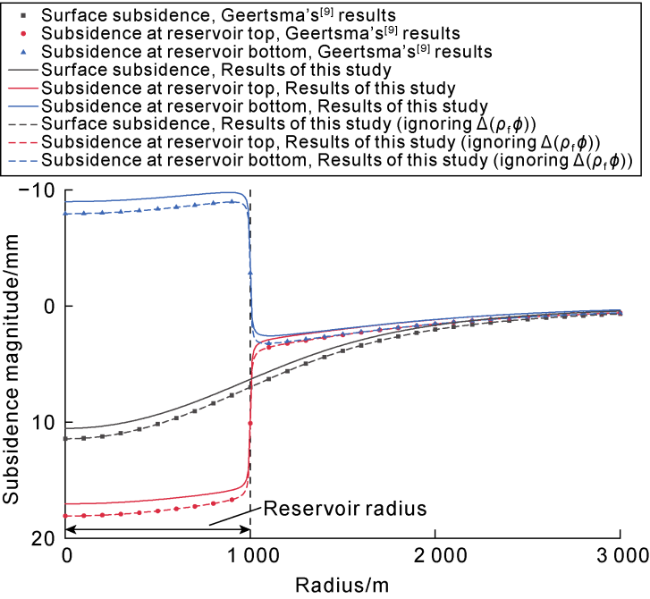
Fig. 4. Comparison of the results of this study with those of Geertsma [9]. |
3.2. Comparative testing with commercial simulator
Consider a homogeneous square reservoir (Fig. 5 ) undergoing depletion development from its initial state to a depleted state. Model parameters are listed in Table 2 , with elastic and other physical properties identical to those in Table 1 .
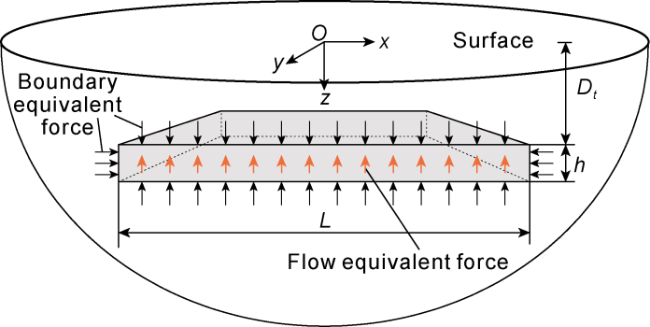
Fig. 5. Homogeneous square reservoir model. |
Table 2. Reservoir parameters for comparative testing |
| Parameter | Value | Parameter | Value |
|---|---|---|---|
| Grid counts (x, y, z) | 20, 20, 5 | Reservoir top depth | 2 000 m |
| Grid sizes (x, y, z) | 100, 100, 2 m | Reservoir side length | 2 000 m |
| Rock bulk density | 2.65 g/cm3 | Initial pressure | 30 MPa |
| Pressure increment | -10 MPa | Reservoir thickness | 10 m |
The VISAGE geomechanical model employs a mesh extension approach to construct its geomechanical grid. Horizontally (x and y-directions), the grid extends outward by more than three times the reservoir dimensions. Vertically upward, it extends to the ground surface. Vertically downward, it reaches a depth sufficient to avoid thin- plate effects, i.e., a thickness no less than one-third of the lateral dimensions (specific parameters shown in Table 3 ). The entire stratum is modeled as a homogeneous, isotropic elastic material with a Biot coefficient of 1-Kp/Ks. A uniform pressure depletion of 10 MPa is applied, with fixed zero-strain boundary conditions except at the ground surface.
Table 3. Parameter settings for the VISAGE model |
| Case | Horizontal extension multiples | Number of horizontal extension meshes | Number of meshes extending above the reservoir | Depth of lower reservoir extension/m | Number of meshes extending below the reservoir |
|---|---|---|---|---|---|
| Case 1 | 3 | 5 | 15 | 6 400 | 20 |
| Case 2 | 10 | 20 | 20 | 15 000 | 50 |
| Case 3 | 30 | 30 | 20 | 30 000 | 70 |
| Case 4 | 100 | 50 | 40 | 140 000 | 90 |
Using Eq. (27), the exact solution for this problem is obtained. For vertical displacement (Fig. 6 ), the exact solution exhibits anomalously low values at the peripheral boundaries in Fig. 6a and anomalously high values at the peripheral boundaries in Fig. 6c , while Fig. 6b shows no significant anomalies. This is because the lateral boundary forces have a minimal impact on the vertical displacement in the middle layer of the reservoir. In this case, the lateral boundary forces are directed inward. These forces induce upward displacement in the upper reservoir and downward displacement in the lower reservoir, creating the peripheral-central discrepancies in Fig. 6a and Fig. 6c . Due to the reservoir’s small thickness relative to its lateral dimensions, the boundary effects are localized, primarily affecting the outermost solution points.
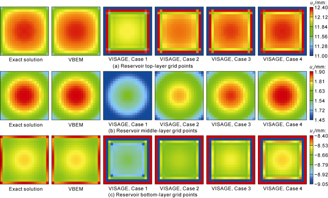
Fig. 6. Comparison of exact solution, VBEM, and commercial simulator results. |
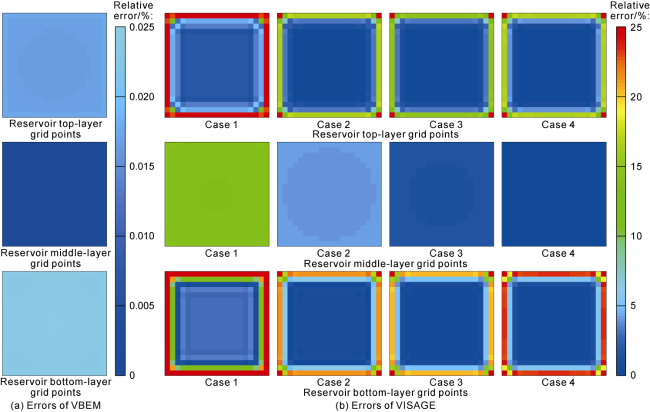
To evaluate the accuracy of different methods, the relative error is defined as the absolute value of the ratio of the difference between the numerical solution and the exact solution to the exact solution. The results of different methods are shown in Fig. 6 , with their relative errors illustrated in Fig. 7. The VBEM developed in this study yields results closely aligned with the exact solution, exhibiting uniformly distributed errors all below 0.025%. VBEM significantly outperforms the commercial simulator VISAGE in accuracy. While VISAGE’s internal reservoir solutions gradually approach the exact solution as the mesh extends, it persistently exhibits large errors at reservoir corner boundaries. For boundary grids at the reservoir top and bottom, relative errors consistently exceed 10%, a level of inaccuracy unacceptable even for engineering applications.
Fig. 7. Comparison of solution errors between the VBEM and commercial simulator. |
The root cause for high errors near flow boundaries in traditional finite element methods (FEM) lies in their theoretical inability to rigorously account for flow boundary effects. Specifically, FEM assumes zero permeability outside reservoir flow boundaries. Initially, pore pressure is mapped from the reservoir flow simulation grid to the finite element grid (reservoir domain) and extrapolated to the extended regions of the 3D finite element mesh. Subsequently, the extended region of the three-dimensional finite element mesh, which is impermeable, maintains a constant pressure. The effect of the flow boundary is reflected through the pressure gradient acting between the reservoir area and the impermeable area. This approach ties boundary effects to mesh properties, resulting in significant errors at boundaries. In contrast, the proposed VBEM circumvents this limitation by directly applying boundary equivalent forces to well-defined boundary surfaces, independent of mesh attributes. Consequently, it achieves numerical accuracy at boundaries consistent with internal regions.
A detailed comparison of solution errors at reservoir grid points across different methods is presented in Table 4 . The results demonstrate that VBEM achieves a maximum error of only 0.024% at reservoir grid points, whereas the commercial simulator VISAGE exhibits maximum errors exceeding 40%. Notably, VISAGE’s maximum error does not decrease with grid extension; instead, its minimum error reduces slightly, offering negligible improvement in result reliability. Additionally, VISAGE’s solution time increases significantly with the grid number. In contrast, VBEM delivers a precision far surpassing the commercial simulator. Compared to VISAGE’s refined Case 4, VBEM reduces the average error in the reservoir region to less than 1/500 of VISAGE’s error, while cutting the solution time by 79%.
Table 4. Performance of simulation methods in solving reservoir grid displacement |
| Solver | Grid number | Solution time/min | Minimum error/% | Maximum error/% | Average error/% |
|---|---|---|---|---|---|
| VBEM | 31.0 | 2.5×10⁻¹⁴ | 0.024 | 0.008 2 | |
| VISAGE (Case 1) | 40 960 | 0.6 | 0.650 00 | 67.210 | 10.770 0 |
| VISAGE (Case 2) | 288 300 | 7.0 | 0.100 00 | 47.380 | 5.150 0 |
| VISAGE (Case 3) | 638 780 | 21.5 | 0.027 00 | 45.360 | 4.050 0 |
| VISAGE (Case 4) | 2 009 340 | 149.2 | 0.000 33 | 51.530 | 4.150 0 |
The proposed VBEM achieves high near-field solution accuracy, and also exhibits the unique advantage of maintaining consistent precision across both near and far field regions. Surface subsidence induced by subsurface reservoir development is a critical focus in geomechanics, necessitating rigorous evaluation of far-field accuracy across methods. Due to differing external grid sizes in the models, comparisons are performed within the reservoir’s vertical projection area at the ground surface. Detailed error comparisons for surface displacement calculations are shown in Table 5 . The results highlight VBEM’s exceptional far-field accuracy: errors are virtually negligible (approaching zero), whereas VISAGE exhibits average errors of 1%-4%, with no significant reduction in far-field errors even after grid extension. Compared to VISAGE’s refined Case 4, VBEM reduces the average far-field error to less than 1/1×1012 of VISAGE’s error.
Table 5. Performance of simulation methods in solving surface subsidence |
| Solver | Top layer grid thickness/m | Minimum error/% | Maximum error/% | Average error/% |
|---|---|---|---|---|
| VBEM | 2.15×10⁻¹³ | 1.95×10⁻¹² | 1.11×10⁻¹² | |
| VISAGE (Case 1) | 668.2 | 0.096 | 2.33 | 1.21 |
| VISAGE (Case 2) | 464.0 | 1.83 | 3.25 | 2.72 |
| VISAGE (Case 3) | 464.0 | 3.00 | 4.08 | 3.68 |
| VISAGE (Case 4) | 216.6 | 1.76 | 2.22 | 2.05 |
Comparative studies based on a uniformly depressurized square reservoir model demonstrate that the VBEM proposed in this work significantly outperforms traditional finite element numerical solvers in solution accuracy. VBEM exhibits superior precision and stability across both reservoir grid points and far-field regions. Notably, commercial simulators like VISAGE universally neglect the influence of dynamic changes in pore fluid density and saturation on strata deformation. Consequently, the exact solution and VBEM model in the above validations also exclude these fluid property variations. When the exact solution accounting for fluid density and saturation changes is taken as the benchmark, traditional commercial simulators exhibit an increase in average error by about 20 percentage points for both reservoir grid points and far-field results (as shown in Table 6 ). In contrast, VBEM fully incorporates these effects, maintaining extremely low error levels throughout. Furthermore, Table 6 reveals that the solution error of commercial simulators at reservoir grid points increases with mesh extension. This counterintuitive trend arises because, as the mesh extends, commercial simulators converge toward solutions that ignore fluid property changes, thereby amplifying deviations from physically realistic results.
Table 6. Solution errors of different methods considering changes in fluid density and saturation |
| Location | Solvers | Minimum error/% | Maximum error/% | Average error/% |
|---|---|---|---|---|
| Reservoir | VBEM | 0.25×10⁻⁴ | 0.023 | 0.008 |
| VISAGE (Case 1) | 0.39 | 83.400 | 25.680 | |
| VISAGE (Case 2) | 2.07 | 103.860 | 29.390 | |
| VISAGE (Case 3) | 0.43 | 109.230 | 30.650 | |
| VISAGE (Case 4) | 1.58 | 112.240 | 31.890 | |
| Surface | VBEM | 4.54×10⁻¹³ | 2.50×10⁻¹² | 1.67×10⁻¹² |
| VISAGE (Case 1) | 18.24 | 18.51 | 18.34 | |
| VISAGE (Case 2) | 19.57 | 21.33 | 20.15 | |
| VISAGE (Case 3) | 20.54 | 22.73 | 21.27 | |
| VISAGE (Case 4) | 18.38 | 21.25 | 19.37 |
4. Conclusions
The effects of internal reservoir flow and flow boundaries on strata deformation are equivalent to the impacts of external forces acting within the reservoir interior and at the reservoir boundaries, respectively. This study provides calculation methods for the flow equivalent force and boundary equivalent force: The flow equivalent force is determined by the pore pressure gradient, fluid mass variation, and rock elastic parameters. The boundary equivalent force is governed by the pore pressure change and rock elastic parameters. The deformation solution at any strata point is obtained through the convolution of the flow equivalent force, boundary equivalent force, and Green’s function. After discretization, the deformation solution is calculated by multiplying grid boundary equivalent forces with corresponding grid boundary sources, grid flow equivalent forces with corresponding grid volume sources, and summing the results. This constitutes the volumetric boundary element method (VBEM).
VBEM offers significant advantages, including eliminating the need for meshing strata outside the reservoir and delivering high solution accuracy. It comprehensively accounts for the effects of reservoir flow boundaries, pore pressure gradient fields within the reservoir, and fluid mass changes in pores on strata deformation. Compared to commercial simulator models, VBEM achieves dramatically improved accuracy, with its precision advantages being particularly pronounced in far-field regions such as the ground surface.
The derivation in this study adopts the assumption of homogeneous strata and does not account for strata heterogeneity or fractures. However, the proposed model exhibits strong extensibility, providing a novel direction for future research. Subsequent work could extend this framework to complex geological settings—such as layered heterogeneous strata and fractured reservoirs—by incorporating modified Mindlin solutions under different assumptions and developing fracture boundary equivalent forces.
Nomenclature
a, b, c—grid cell indices in the x, y, z-directions (increasing with coordinate axes);
A—cross-sectional area of the element, m2;
Ct—total compressibility, Pa-1;
D—depth, m;
Dt—depth to reservoir top, m;
fi—total external force per unit apparent volume on the rock skeleton in the i-direction, Pa/m;
fe,i—flow equivalent force in the i-direction, Pa/m;
Fi—body force in the i-direction exerted by fluid on the skeleton, Pa/m;
$\tilde{F}_{i j}$—grid boundary source, m3/N;
grid(a, b, c)—grid cell with indices a, b, c in x, y, z-directions;
G—apparent shear modulus of the rock, Pa;
g—gravitational acceleration, m/s2;
h—reservoir thickness, m;
Kp—apparent bulk modulus of the rock, Pa;
Ks—bulk modulus of the skeleton material, Pa;
L—reservoir length, m;
, —unit inward normal vectors at closed boundary Γ for internal and external domains;
p—pore fluid pressure, Pa;
p0—initial pressure, Pa;
R—reservoir radius, m;
ui—displacement of the rock in the i-directions, m;
$\tilde{u}_{i j}$—displacement Green’s function, m/N;
$\tilde{V}_{i j}$—grid volume source, m4/N;
x, y, z—cartesian coordinates, m;
xi—coordinate in the i-direction, m;
Δxi—length of the element, m;
Δx, Δy, Δz—grid cell sizes in x, y, z-directions, m;
α, β, γ—coordinates of an arbitrary point in the strata, m;
Γ—closed boundary;
δij—kronecker delta, δij=0 if i≠j, δij=1 if i=j;
ε—apparent volumetric strain of the rock, dimensionless;
$\varepsilon_{i j}$—apparent strain of the rock, dimensionless;
$v$—apparent Poisson’s ratio of the rock, dimensionless;
$\rho_{\mathrm{f}}$—average density of fluid in rock pores, kg/m3;
$\rho_{\mathrm{s}}$—density of the skeleton material, kg/m3;
\rho_{\mathrm{ref}—average fluid density at reference pressure, kg/m3;
$\bar{\rho}$—average density of fluid-saturated rock, kg/m3;
σij—skeleton stress of the rock (positive for tension, negative for compression), Pa;
σs,ij—true skeleton stress, Pa;
σt,ij—total stress of saturated rock, Pa;
ϕ—rock porosity, %;
Ω—internal domain bounded by closed boundary;
—external domain bounded by closed boundary.