

Introduction
Worldwide development practices have shown that the multi-staged fracturing technology of long horizontal wells is the key for achieving commercial development of tight oil and gas reservoirs [1-2]. However, due to reservoir stress, rock anisotropy, and interference of artificial fractures [3-5], the created fractures often have significant differences in their locations, fracture length, and leakoff rates compared to the design scheme [6], which affects the fracturing effect and development efficiency. Accurately monitoring and characterizing the fracture parameters during the multi-staged fracturing treatments along horizontal wells, for real-timely optimizing the fracturing design and adjusting the fracturing operation, is crucial to improve the fracturing effect. Currently, it is still a technical challenge.
Limited by the costs, accuracy, and tools, conventional monitoring methods such as chemical tracer, microseismic mapping, pressure transient analysis, and downhole imaging cannot precisely diagnose the dynamic parameters of multi-cluster fracture propagation during the fracturing treatments [7-10]. In recent years, a new diagnostic technology for hydraulic fracture propagation has emerged and played an important role in fracturing-operation monitoring in the United States [11]. Its principle is to monitor the temperature response data along the horizontal wellbore during the multi-staged fracturing treatments through distributed temperature sensing (DTS), and then combine the temperature forward model and inversion method to diagnose the dynamic fracture parameters during the fracturing operation [12].
Many scholars established the forward models to simulate the temperature behavior during the fracturing treatment. Kamphuis et al. [13] built a temperature model of vertical well during fracturing operation considering heat conduction and convection, and predicted the temperature distribution of fractures and formations. Seth et al. [14] constructed a numerical model of temperature response during fracturing treatments in vertical well utilizing finite difference method and Carter model. Hoang et al. [15] proposed a temperature numerical method for the limited-entry fracturing treatment. Li and Zhu [16] presented a thermal model predicting temperature distribution along the wellbore for a single-stage fracturing treatment. Clearly, current temperature forward models are mostly designed for the temperature behavior of single hydraulic fracture, while temperature models for multi-staged hydraulic fracturing processes are rarely reported. Recently, China has conducted field-scale experiment using DTS as monitoring tool during multi- staged fracturing treatments along horizontal wells in multiple oilfields, and obtained a large amount of temperature measurements [17-18]. However, the progress in data interpretation lags behind the advancements in DTS testing technology, limiting the application of DTS in real-time diagnosis of fracture parameters during fracturing operation. Moreover, the existing models cannot take into account the short pump shut-in period during the fracturing operation, making it difficult to adapt to the real conditions on site.
This work first presents a thermo-fluid coupling forward model for multi-staged fracturing of horizontal wells with consideration of the temporary pump shut-in condition during fracturing treatments. Then, the effects of key fracturing and fracture parameters on DTS temperature behavior are identified by a sensitivity analysis. Moreover, an inversion model based on the simulated annealing algorithm is presented to diagnose the fracture parameters. Finally, the reliability of the presented model is verified through a field case study.
1. Thermo-fluid coupling forward model for multi-staged fracturing of horizontal wells
1.1. Physical model
As shown in Fig. 1 , the hydraulic fracturing process starts from Stage 1, and the remaining stages along the horizontal wellbore are sequentially stimulated. During the fracturing of each stage, multiple clusters of fractures are created, and packers prevent fracturing fluid from entering other stages. During the injection period, fracturing fluid continuously enters the wellbore to create hydraulic fractures, and leak off into the reservoir. The fracturing fluids cool the wellbore, fractures, and reservoir due to the heat conduction and convection. During the shut-in period, the fracturing fluid injection stops. The wellbore, fractures, and reservoir begin to warm back under the effect of heat conduction from the reservoir. Throughout the entire process, DTS installed outside the casing monitors the real-time temperature profile along the horizontal wellbore.
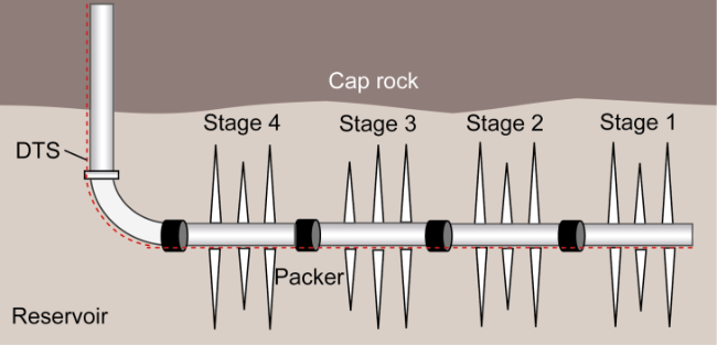
Fig. 1. Sketch of the temperature monitor using DTS during multi-staged fracturing of horizontal wells. |
The physical description of a repetitive element of one stage is presented to develop a model for understanding the DTS temperature behavior during multi-staged fracturing treatment along horizontal wells. Multi-staged hydraulic fracturing treatments considered here encompass the fluid flow and heat transfer in wellbore, fracture propagation, and fracturing fluid leakage (Fig. 2 ).
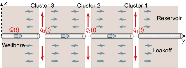
Fig. 2. Sketch of the fracturing fluid flow and leak-off. |
The modeling is based on the following assumptions:
(1) The reservoir is a porous medium with initial temperature Ti, thickness h, and effective porosity ϕ, as well as closed top and bottom boundaries.
(2) The incompressible fracturing fluid is injected into the reservoir at a total flow rate Q(t), creating N clusters of hydraulic fractures. The flow rate of nth cluster is qn(t).
(3) The hydraulic fractures fully penetrate the reservoir and are symmetrical to wellbore. The fracture width and half-length are wn and xf,n, respectively.
(4) There is a pump shut-in with duration tc during multi-staged fracturing treatments.
(5) The leakoff of fracturing fluid is considered as a linear flow perpendicular to the fracture face. The classical Carter model is employed to represent this leakage [19]. The leak-off coefficient of any given cluster n is Clk,n.
(6) The fracture is considered as two-dimensional propagation with constant height.
1.2. Mathematical model
Consider the fluid flow and heat transfer in the wellbore, fracture, and reservoir, the thermo-fluid coupling models are established for injection and shut-in periods to simulate the temperature behavior during multi-staged fracturing treatments along horizontal well.
1.2.1. Wellbore flow model
The governing equation of incompressible fluid flow in horizontal wellbore is derived based on the conservation of mass, as given by:
The initial conditions are:
The boundary conditions are:
1.2.2. Wellbore temperature model
The wellbore temperature equation considering the fracture locations is presented during the injection period based on the mass, energy, and momentum conservation, as given by [20]:
The initial and boundary conditions are:
During the shut-in period, the dominating mechanism is the heat conduction [21] and the wellbore temperature equation is derived based on the energy conservation.
The wellbore temperature at the moment of shut-in is considered as the initial condition for Eq. (6). The boundary conditions without flow and heat transfer are applied.
1.2.3. Fracture propagation model
Carter model [19] is employed to represent the hydraulic fracture propagation. Considering half of the fracture length due to the symmetry assumption, the fracture propagation model can be written based on mass conservation as:
Considering the shut-in condition, the leakoff velocity of fracturing fluid is defined as:
1.2.4. Fracture temperature model
Considering the heat conduction and convection at x- and y- direction caused by the flow and leakage of fracturing fluid, the fracture temperature model during injection period is derived based on energy conservation and Newton’s cooling law [22], as given by:
The initial and boundary conditions are:
During the shut-in period, the flow velocity of fracturing fluid equals 0. Fracture temperature model is presented based on Fourier's law of heat conduction, as given by:
where the fracture temperature at the moment of shut-in is the initial condition for Eq. (11).
1.2.5. Reservoir flow model
A linear leakoff of fracturing fluid from the fracture to the reservoir takes place. Considering the reservoir is a porous medium with porosity ϕ, the actual leakoff distance is described as:
1.2.6. Reservoir temperature model
The reservoir is divided into two zones based on whether or not it is affected by fracturing fluid leakoff. In the reservoir zone affected by the fracturing fluid leakoff, the governing equation describing the reservoir temperature behavior during the injection period is given as:
where
The initial conditions are:
The boundary conditions are:
In the reservoir zone not affected by the fracturing fluid leakoff, the governing equation is derived considering heat conduction to describe the reservoir temperature behavior during the injection period, which can be also used to describe the temperature behavior during the shut-in period.
where
The initial conditions are:
The boundary conditions are:
1.3. Numerical solution procedure
A procedure is presented to numerically solve the temperature model due to the complicated nonlinear component. The whole domain, including the wellbore, fracture and reservoir, is discretized into grids, as shown in Fig. 3. The wellbore is represented by the blocks in the first row. Constant time step size is used in numerical solution. Three indices (i.e., i, j, k) are used to represent the grid points of the x-direction, y-direction, and time domain, respectively. Additionally, two difficulties need to be considered. First, the hydraulic fracture length and fluid leakoff distance dynamically increase during fracturing operation. The fracture and reservoir grids need to be updated for different time steps during numerical computation. Second, different clusters of fractures are subjected to different flow rates of fracturing fluid during the treatment, leading to different fracture propagation lengths at the same time step. Grid remeshing is necessary for fractures with extended fracture lengths to maintain a uniform grid for all clusters in the numerical computation time step. As shown in Fig. 3 , grid remeshing is performed for Cluster 3 of fractures according to the fracture length of Cluster 1 and Cluster 2.
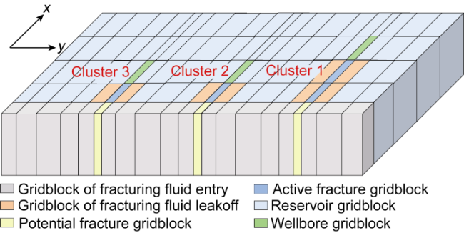
Fig. 3. Grid remeshing of wellbore, fracture and reservoir. |
1.3.1. Grid size
The grid size at x- and y-direction is determined by discretizing Eq. (7) and Eq. (12).
It should be noted that using Eq. (19) can only obtain the fracture length at every time step. Grid remeshing based on Eq. (19) needs to be performed to determine the x-direction grid size (i.e., Δxn,i).
1.3.2. Wellbore equation discretization (injection period)
Discretizing Eq. (4) yields:
v and vi in Eq. (21) are determined by discretizing Eq. (1) and Eq. (3).
1.3.3. Fracture equation discretization
Discretizing Eq. (9) yields:
vx and vlk in Eq. (22) are determined by discretizing Eq. (7) and Eq. (8).
1.3.4. Reservoir equation discretization
Discretizing Eq. (13) yields:
Using the same method for Eq. (16) yields the discretization form of reservoir equations for the reservoir zone not affected by the fracturing fluid leakoff and shut-in period, respectively.
Finally, the temperature behavior during the multi- staged fracturing treatment along horizontal wells can be obtained by solving the discretization equation system using commonly-used Newton's iterative method, which can be implemented using toolbox in MATLAB or Python.
1.4. Inversion model of fracture parameters
An inversion objective function is constructed using the theoretical temperature calculated by forward model and DTS measurements, as given by:
Inversion is the process of iterating and updating the target parameter A until the calculation results satisfy Eq. (24). This process is completed using simulated annealing algorithm in five steps (Fig. 4 ):
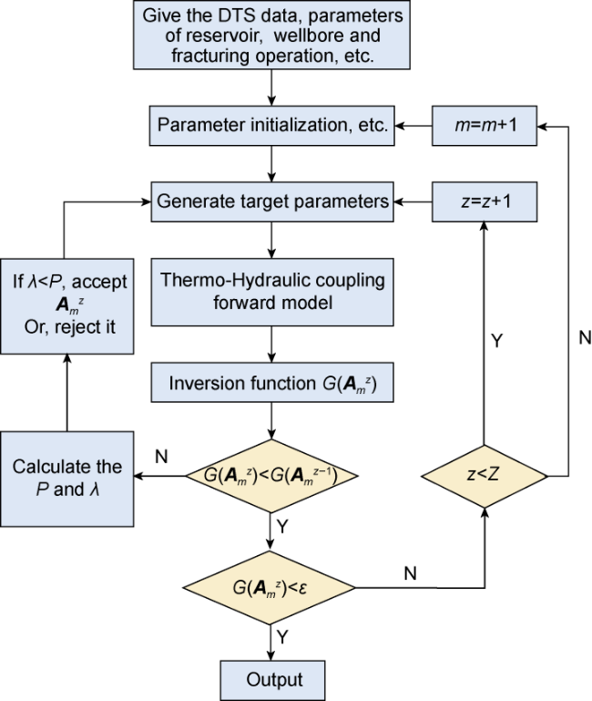
Fig. 4. Inversion procedure based on simulated annealing algorithm. |
(1) Initialize the annealing temperature T0, target parameters , and Markov chain length LN;
(2) Generate new target parameters by Eq. (25) for the zth iteration under the annealing temperature Tm and calculate the temperature response Tp by the forward model;
(3) If , then is final values of target parameters; otherwise, calculate the Metropolis probability P by Eq. (26) and generate a uniformly distributed random number λ in the interval . If λ<P, then accept as the values of target parameters; otherwise, reject it;
(4) Repeat Step (2) by Z times at the annealing temperature Tm until a complete Markov chain is generated;
(5) If , it indicates that the inversion has converged, and the algorithm ends. Otherwise, a new annealing temperature and chain length will be generated based on Eq. (27). The process will proceed to Step (2) until , then, the results are output.
2. Sensitivity analysis
To better understand the temperature behavior along a horizontal wellbore during the hydraulic fracturing process, the impacts of fracturing parameters (i.e., fracturing fluid flowrate, injection time and shut-in time) and fracture parameters (i.e., fracture width and leakoff coefficient) on DTS measurements are simulated by the presented forward model with consideration of both injection (120 min) and short shut-in periods. The fundamental parameters are listed in Table 1 . The cluster spacing is set to 10 m. Considering that the time step will affect the grid number and temperature results, a sensitivity analysis of time step size (5, 10, 15 min) is conducted for determining a reasonable time step size so that ensure the calculation results are independent of the grid number. As shown in Fig. 5 , the temperature calculation results are independent of the grid number under the given time step size. Therefore, the time step size for temperature simulation is set to 10 min in this study.
Table 1. Basic parameters for temperature simulation |
| Parameter | Value | Parameter | Value |
|---|---|---|---|
| Initial temperature | 90 °C | Fracture width | 0.006 m |
| Porosity | 5% | Fracture height | 30 m |
| Thickness | 30 m | Newton’s cooling coefficient | 50 W/(m2·K) |
| Rock density | 2 381 kg/m3 | Leakoff coefficient | 5×10⁻⁴ m/s0.5 |
| Rock heat capacity | 844 J/(kg·K) | Wellbore radius | 0.1 m |
| Rock heat conductivity | 2.596 W/(m·K) | Overall heat transfer coefficient | 30 W/(m2·K) |
| Reservoir fluid density | 913 kg/m3 | Pumping flowrate | 0.2 m3/s |
| Reservoir fluid specific heat capacity | 4 136 J/(kg·K) | Fracturing fluid temperature | 10 °C |
| Reservoir fluid heat conductivity | 0.156 W/(m·K) | Fracturing fluid density | 986 kg/m3 |
| Fracturing fluid heat conductivity | 0.606 W/(m·K) | Fracturing fluid heat capacity | 4 136 J/(kg·K) |
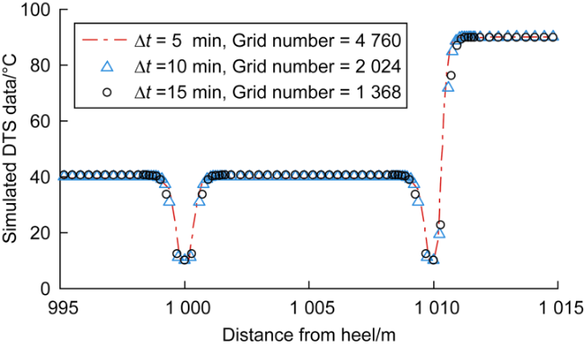
Fig. 5. Simulated temperatures at different time step sizes and grid numbers. |
2.1. Impact of fracturing time
Four cases of different fracturing time (60, 80, 100, 120 min) are designed to investigate the effects on temperature distribution. The fracturing fluid flowrate is given a constant value of 0.1 m3/s without consideration of the shut-in period. As shown in Fig. 6 , as fracturing time increases, the fracture length and the distance of fracturing fluid leakoff to the reservoir increase, leading to the low-temperature zone expansion. Moreover, in Fig. 7 , the temperature curve exhibits a V-shaped pattern. As the fracturing time increases, the V-shape decreases in depth and increases in width. The V-shape position and number correspond to those of the created fractures.
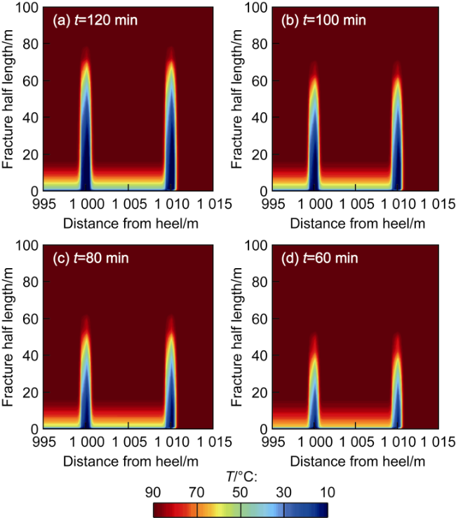
Fig. 6. Temperature distribution under different fracturing time during multi-staged fracturing treatment along horizontal well. |
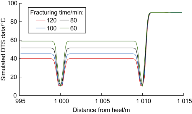
Fig. 7. DTS measurements under different fracturing time during multi-staged fracturing treatment along horizontal well. |
2.2. Impact of shut-in time during fracturing operation
Different shut-in time (0, 10, 20, 40 min) are designed to investigate the effects on temperature distribution. The fracturing fluid flowrate is considered a constant value of 0.1 m3/s and fracturing time is 120 min. In Fig. 8 , no obvious difference occurs in the temperature distribution as the shut-in time increases. However, in Fig. 9 , the temperature and the V-shape depth decrease. This is because the low-temperature fluids continuously cool the wellbore, and the reservoir needs more time to warm the wellbore. Therefore, during the short shut-in period, the cooling effect of fracturing fluids still spreads to the reservoir, and the temperature near the wellbore decreases instead of rise. This is different from the traditional understanding.
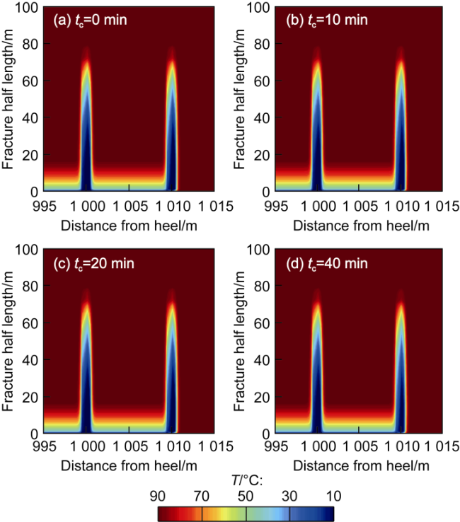
Fig. 8. Temperature distribution under different shut-in time during multi-staged fracturing treatment along horizontal well. |
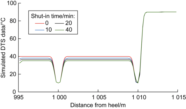
Fig. 9. DTS measurements under different shut-in time during multi-staged fracturing treatment along horizontal well. |
2.3. Impact of fracturing fluid flowrate
The effects of different fracturing fluid flowrates (i.e., 0.10, 0.05, 0.03, 0.01 m3/s) on temperature distribution are investigated. q1 is considered a constant value of 0.1 m3/s and the fracturing time is 120 min without consideration of shut-in period. As shown in Fig. 10 and Fig. 11 , with the increase of fracturing fluid flowrate, the fracture length increases and the low-temperature zone expands. Moreover, the DTS temperature curve shows a lower position, and the V-shape depth decreases. However, the fracturing fluid flowrate has no effect on the V-shape width.
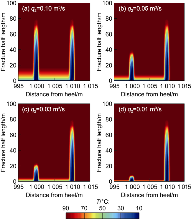
Fig. 10. Temperature distribution under different fracturing fluid flow rates during multi-staged fracturing treatment along the horizontal well. |
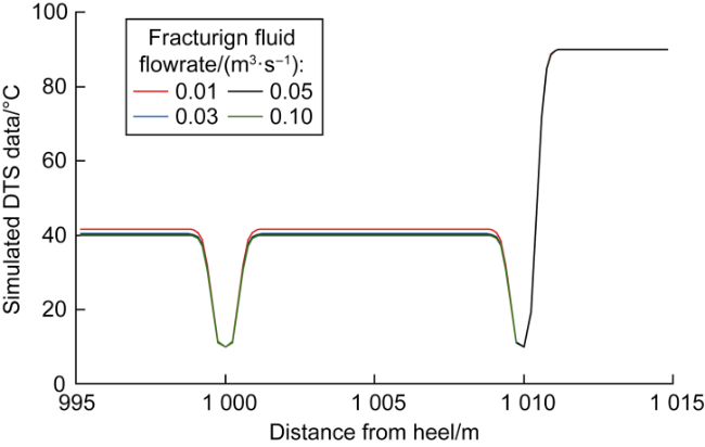
Fig. 11. DTS measurements under different fracturing fluid flowrates during multi-staged fracturing treatment along horizontal well. |
2.4. Impact of fracture width
The effects of different fracture widths (0.003, 0.006, 0.009, 0.012 m) on temperature distribution are investigated. The fracturing fluid flowrate is considered a constant value of 0.1 m3/s and the fracturing time is 120 min without consideration of shut-in period. As shown in Fig. 12 and Fig. 13 , the low-temperature zones in and around fracture shrink with the increase of fracture width. Moreover, the V-shape width of the DTS temperature curve decreases.
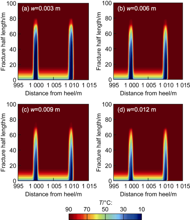
Fig. 12. Temperature distribution under different fracture widths during multi-staged fracturing treatment along the horizontal well. |
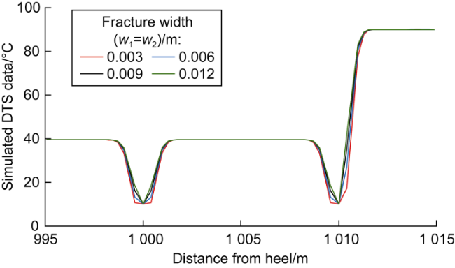
Fig. 13. DTS measurements under different fracture widths during multi-staged fracturing treatment along horizontal well. |
2.5. Impact of leakoff coefficient
The effects of different leakoff coefficients 5×10⁻⁴, 7× 10⁻⁴, 9×10⁻⁴, 11×10−4 m/s0.5 on temperature distribution are investigated. The fracturing fluid flowrate is considered a constant value of 0.1 m3/s and the fracturing time is 120 min without consideration of shut-in period. As shown in Fig. 14 and Fig. 15 , as the leakoff coefficient increases, the low-temperature zone shrinks in the fracture and expands around the fracture, while the temperature field in the reservoir becomes lower and wider. Moreover, the V-shape width of the DTS temperature curve increases.
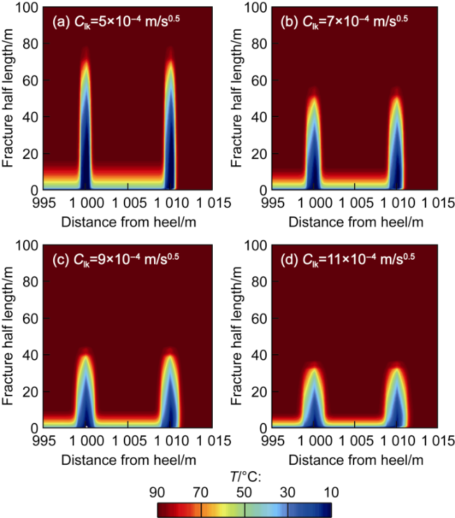
Fig. 14. Temperature distribution under different leakoff coefficients during multi-staged fracturing treatment along the horizontal well. |
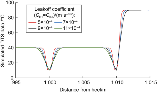
Fig. 15. DTS measurements under different leakoff coefficients during multi-staged fracturing treatment along horizontal well. |
3. Field case study
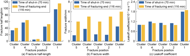
The horizontal well X15-4 targeting shale oil reservoirs in the Qaidam Basin, with the depth of 5 176 m, effective horizontal section length of 1 552 m, reservoir thickness of 10.3 m, and reservoir porosity of 5.12%, is chosen for case study of multi-staged fracturing stimulation. The fracturing scheme is designed with 27 stages of fractures, 3-8 clusters of fractures for each stage, and a total fracturing fluid flowrate of 14-18 m3/min. The total fracturing time is 100 min, with a shut-in for 16 min at 70 min of fracturing operation. The temperature response during the fracturing operation is monitored using DTS with a depth of 5 176 m and covering the entire wellbore. The spatial resolution is 0.25 m, and the temporal resolution is 30 s. The DTS temperature data during the fracturing process is shown in Fig. 16a . The original data was further denoised as given in Fig. 16b . The 26th stage is designed with 5 clusters of fractures, with an injection flowrate of 0.268 m3/s. The DTS temperature data at the time of shut-in (70 min) and the end of fracturing operation (116 min) is respectively interpreted using the proposed method.
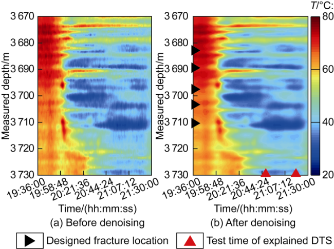
Fig. 16. Waterfall plot of DTS temperature data recorded during fracturing operation. |
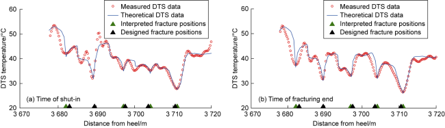
Fig. 17. Matching with DTS measurements. |
Fig. 18. Interpretation of fracture parameters at the time of shut-in and fracturing end. |
4. Conclusions
The DTS temperature curve during multi-staged fracturing treatment along horizontal well typically exhibits a V-shaped pattern. Its position and number correspond to those of the created fractures. Based on this observation, the location and number of the created fractures can be directly identified from DTS temperature curve.
The DTS temperature curve is lower in position for a higher fracturing fluid flowrate, longer fracturing time and longer shut-in time, leading to a smaller V-shape depth. Also, a wider V-shape appears for a higher leakoff coefficient, longer fracturing time and smaller fracture width. During the shut-in period, the low temperature still spreads to the reservoir, and the temperature near the wellbore decreases instead of rising.
The fracture parameters during fracturing operation of a multi-staged fractured horizontal well can be determined by interpreting DTS data, which can be used to diagnose the fracture propagation during fracturing operation and take prompt measures for improving the fracturing effects.
Nomenclature
A—parameter vector to be inverted;
—initial parameter vector to be inverted;
Clk—leakoff coefficient, m/s0.5;
Clk1, Clk2—leakoff coefficient of fractures in clusters 1 and 2, m/s0.5;
cpf—reservoir fluid capacity, J/(kg·K);
cpl—fracturing fluid capacity, J/(kg·K);
cps—rock capacity, J/(kg·K);
g—gravitational acceleration, m/s2;
G(A)—inversion objective function, K;
h—fracture height, m;
hl—Newton’s cooling coefficient, W/(m2·K);
i—x-direction grid points;
j—y-direction grid points;
k—time-domain grid points;
kb—Bolzamann constant, J/K;
LN—Markov chain length;
Llk—leakoff distance, m;
m—the mth annealing;
n—fracture cluster number;
N—total clusters of hydraulic fracture;
P—Metropolis probability, dimensionless;
Q—total fracturing fluid flowrate, m3/s;
q—fracturing fluid flowrate of single cluster fracture, m3/s;
q2—fracturing fluid flowrate of Cluster 2 fracture, m3/s;
rw—horizontal wellbore radius, m;
t—fracturing time, s;
tc(x)—the time duration of shut-in (the pump stops at location x on the fracture surface), s;
T0—initial annealing temperature, K;
Ti—initial reservoir temperature, K;
Tinj—fracturing fluid injection temperature, K;
Tw—wellbore temperature, K;
Tf—fracture temperature, K;
Tr—reservoir temperature, K;
—calculated theoretical temperature, K;
Tm—temperature measured by DTS, K;
Tm—mth annealing temperature, K;
UT—overall heat transfer coefficient, W/(m2·K);
v—flow velocity in the wellbore, m/s;
vi—velocity injecting into fracture, m/s;
vlk—leakoff velocity, m/s;
vx—fracturing fluid velocity in fracture, m/s;
w—fracture width, m;
w1, w2—fracture width of clusters 1 and 2, m;
xf—fracture half length, m;
xe, ye—reservoir boundary, m;
x, y—x and y coordinate, m;
Δx—x-direction gridsize, m;
Δy—y-direction grid size, m;
yf-r—position between fracture and reservoir, m;
z—the zth inversion;
Z—total inversion iteration number;
α—temperature decay rate, 0.1;
γ—the ratio of pipe open area to the total area (γ=1 in fracture position, γ=0 in other positions);
Δt—time step size, s;
ε—inversion error tolerance, dimensionless;
ζ—disturbance coefficient, 0.1;
θ—horizontal wellbore incline, (°);
λ—uniformly distributed random number, dimensionless;
λ1—fracturing fluid heat conductivity, W/(m·K);
λef—average heat conductivity of reservoir zone not affected by fracturing fluid leakoff, W/(m·K);
λel—average heat conductivity of reservoir zone affected by fracturing fluid leakoff, W/(m·K);
ρ1—fracturing fluid density, kg/m3;
ρi—fracturing fluid density injecting to fracture, kg/m3;
ρf—reservoir fluid density, kg/m3;
ρs—rock density, kg/m3;
τ(x)—the time at which the fracturing fluid leakoff begins at location x on the fracture surface, s;
ϕ—reservoir porosity, %.