

Introduction
In the early development stage of a shale gas field in the eastern Sichuan Basin, SW China, the well spacing ranged from 500 m to 600 m, but subsequent evaluations confirmed the existence of unstimulated blank zones between wells[1]. To enhance stimulated reservoir volume (SRV) and natural gas production, the field initiated a cube development test in 2018, reducing well spacing to 300 m. The infill well tests demonstrated that commercial production could be achieved by vertically dividing the Silurian Longmaxi Formation into three sections for cube development [2]. Following the successful tests, multiple shale gas fields including Changning, Luzhou, Zhaotong, and Weiyuan began feasibility assessments of the cube development [3-6]. In North America, the cube development of "multi-stacks, multi-layers" shale formations typically achieves effective reservoir development through one-time deployment of well groups during early stages. In contrast, the shale gas reservoirs in the Sichuan Basin feature older geological age, greater burial depth, strong heterogeneity, developed beddings/faults, and complex and diverse spatial distribution of in-situ stress fields. These distinctive geological characteristics result in a "single-stack, multi- layers, multi-periods" development pattern for cube development infill well pads in the Sichuan Basin. For some well groups with long production histories, the time interval between initial drilling and infill well deployment can reach 5-10 years. During this period, the production of parent wells leads to reservoir pressure depletion, which changes both the direction and magnitude of in-situ stress, thereby affecting fracture propagation and reservoir stimulation effectiveness. When designing well pattern and fracturing parameters for infill wells, the initial stress field cannot be used as the basis. Instead, it is necessary to characterize the four-dimensional in-situ stress evolution (three-dimensional reservoir space + time dimension) in complex natural fracture reservoir [7-9]. This represents the most distinctive difference between hydraulic fracturing in infill wells versus other shale gas wells. With the deployment of infill wells and the decreasing of well spacing, issues such as well pattern, well spacing and prevention of inter-well interference must be reconsidered [10-16]. In studies of dynamic stress field evolution, scholars currently widely employ the finite element method coupled with finite difference or finite volume methods for seepage-stress coupling calculations. The coupling approaches mainly include fully coupled, iteratively coupled, and one-way coupled schemes [17-20]. These methods have been primarily applied to conventional reservoirs [21-22] and fractured reservoirs [23] to establish four-dimensional in-situ stress evolution models. However, these existing models fail to account for reservoir heterogeneity. Regarding hydraulic fracturing and inter-well interference in cube development well pads, the primary research focus lies in determining optimal well spacing, well pattern and fracturing parameters to maximize stimulated reservoir volume (SRV) and production rate [10-23]. Although there have been many simulation studies on the hydraulic fracturing of infill wells, few simulation studies at the scale of cube development infill well groups have been conducted, taking into account reservoir stress evolution and complex fracture propagation.
Aiming at the problems of inter-well interference prevention and fracturing parameter optimization faced by the "multi-layers, multi-periods" development of the X1 infill well pad, this paper proposes a fracturing simulation method for cube development infill well pads considering four-dimensional in-situ stress evolution, and explores the inter-well interference mechanism and the optimal combination of well pattern, well spacing, and fracturing parameters. Compared with the authors previous research on single-layer infill well pad [7], this study has made significant progress in methods, dimensions, and theories: (1) Based on the existing theoretical models, we considered reservoir anisotropy and effects of stress disturbance during fracturing to develop a multi-field coupled theoretical model accounting for hydraulic/natural fracture interactions and fracturing stress disturbance. (2) Considering geological variations, we modeled the high-strength limestone interbed at the top of the Longmaxi Formation and the natural fracture zones running through the reservoir, enhancing model complexity and resolution. (3) By developing new interface programs, we achieved efficient integration among Petrel RE, Fracman, and ABAQUS, upgrading the simulation methodology. (4) The research scope expanded from planar to cube development, incorporating both vertical and horizontal interference while covering broader spatial-temporal domains. In addition, three inter-well interference modes were identified: frac-hit, communication through natural fractures, and pressure/stress interference. (5) Two inter-well interference mechanisms, namely communication of natural fractures and disturbance of in-situ stress field were revealed, and a 5-step progressive optimization process of fracture inversion, history matching, in-situ stress prediciton, fracture design and productivity optimization targeting inter-well interference control and productivity maximiation was proposed.
1. Fracturing simulation for cube development infill well pads based on 4D in-situ stress evolution
1.1. Simulation of infill well fracturing
The multi-field coupled simulation and optimization methodology for infill well hydraulic fracturing was proposed based on the geology-engineering integration concept: (1) Integrated geological modeling: Seismic, geological, and well-logging data were integrated to construct a comprehensive geological model incorporating a discrete fracture network (DFN), to characterize shale reservoir heterogeneity and fracture features. (2) Parent well hydraulic fracturing simulation: A hydraulic fracturing model combining DFN and the finite element method (FEM) was employed to inversely simulate fracture geometry based on field fracturing parameters from parent wells. (3) Four-dimensional in-situ stress evolution prediction: A finite difference seepage and finite element geomechanics coupling model was constructed. Based on Oda’s method [24], the hydraulic fracture parameters of parent wells were transmitted to the seepage model, and the formation pressure changes were inverted through history matching of parent well production data. Porosity, permeability, and pore pressure were cross-iteratively coupled between the seepage model and the geomechanics model. Four-dimensional in-situ stress evolution prediction was achieved through secondary development of Petrel RE, Fracman, and ABAQUS software platforms. (4) Hydraulic fracturing simulation and parameter optimization of infill well: Based on the updated stress field, fracturing parameters for infill wells were optimized to maximize SRV and well pad productivity while avoiding inter-well interference.
1.2. Governing equations of hydraulic fracturing and seepage-stress coupling process
1.2.1. Governing equations of hydraulic fracturing
The hydraulic fracturing simulation is based on the DFN model and adopts the critical stress analysis theory to solve the constitutive relationship of fluid mass conservation on a random fracture network. After fracturing fluid injection, when the fracture initiation conditions are met, hydraulic fractures propagate parallel to the direction of the maximum horizontal principal stress. During their propagation, the natural fractures along the extension direction are real-time detected to determine whether they allow fracturing fluid entry. Corresponding fractures are activated when the pressure within natural fractures reaches the instability condition. This simulation method requires maintaining the volume balance of the fracturing fluid with hydraulically expanded fractures and activated natural fractures, thereby achieving the simulation of hydraulic fracture propagation. The fracture expansion is related to the elastic properties of the rock, stress state, and internal fracture pore pressure. The mass conservation relationship of the fluid can be expressed as:
As the fracturing fluid is injected, the pressure inside the wellbore continuously increases. When the tensile stress around the well is greater than the tensile strength of the rock, the hydraulic fractures begin to propagate in the form of expansion at the borehole [7]. This criterion can be expressed as:
$\sigma_{\mathrm{w}}>\sigma_{\mathrm{T}}$
After the fracture is opened, the fluid continues to flow into it. Considering the frictional resistance on the fracture surface and the fluid leak off, the fluid pressure inside the expanding fracture can be expressed as:
$p_{\mathrm{frac}}=\left(p_{\mathrm{pu}}-\sigma_{\mathrm{N}}\right)\left(1-s \frac{d}{d_{\max }}\right)+\sigma_{\mathrm{N}}+\rho_{\mathrm{L}} g H$
The shear failure of natural fractures can be judged by the Mohr-Coulomb criterion [7], which can be expressed as:
After the fracture initiation, the simulation of fracture propagation is based on the Secor and Pollard method [25]. The fracture width can be calculated by the following formula:
During the iterative process of fracture propagation simulation, the fracture height is a preset parameter, and the fracture length is obtained through iterative calculation by maintaining the balance between the volume of the fracturing fluid and the volumes of the hydraulic fractures and the activated natural fractures. The specific iterative process can refer to the Reference [18].
1.2.2. Governing equations of seepage-stress coupling process
Shale gas differs from conventional natural gas in terms of storage mode and seepage characteristics. In shale gas production, it is essential to account for gas adsorption/desorption, slippage effects, and Knudsen diffusion. These phenomena are typically characterized using the Langmuir isothermal adsorption equation and apparent permeability [26]. Shale reservoirs exhibit well-developed natural fractures, displaying characteristic dual-porosity media behavior for gas transport. Consequently, a dual-porosity dual-permeability model was employed in the flow simulation. Within this matrix-fracture flow system, gas transport equations are formulated separately for both the matrix and fracture systems. The equation for the gas seepage velocity in the matrix can be expressed as:
In natural fractures and hydraulic fractures, the gas seepage velocity equation is described by Darcy's law:
The material balance equation for natural gas in the matrix, natural fractures, and hydraulic fractures can be expressed as:
For the solid medium of shale, the effective stress and principal stress of poroelastic shale follow Biot’s effective stress theory [27], and its stress equilibrium equation can be expressed as:
The stress-strain relationship can be given by Hooke’s law formula:
2. Model establishment and verification
2.1. Geological-engineering background of Well Pad X1
The shale gas field is located in the Wanxian Syncline within the high-steep fold belt of the eastern Sichuan Basin. Its main reservoirs are Ordovician Wufeng Formation to Silurian Longmaxi Formation (burial depth: 2 300-2 500 m), and is subdivided into nine sub-layers (①-⑨) across top, middle, and bottom sections. Well pad X1 employs a three-layer cube development approach comprising nine horizontal wells, utilizing a multi-layer, multi-period infill development strategy. Early in the development process, only the parent well B1 was put into production. Subsequently, infill wells were gradually drilled in different sections. Spatially, the infill wells traverse the top, middle, and bottom sections of reservoir. Temporally, drilling and fracturing were implemented in four periods. The well location relationships and production sequence are shown in Fig. 1.
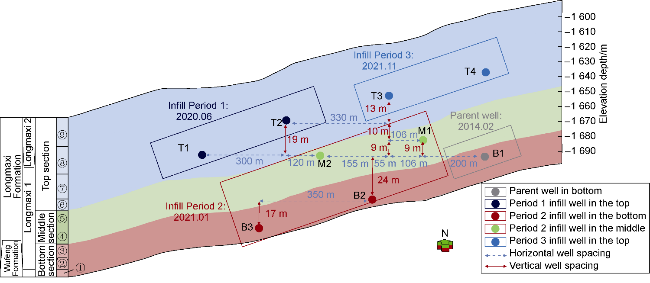
Fig. 1. Schematic of the well location relationship and development time sequence of Well Group X1. |
2.2. Parameters of the model
According to the requirements of four-dimensional in-situ stress and hydraulic fracturing simulation of infill wells, a comprehensive numerical model of well pad X1 was established. The main geological parameters and hydraulic fracturing parameters of the parent well and Period 1 infill wells are shown in Table 1.
Table 1. Main parameters of the model |
| Parameter name | Value | Parameter name | Value | Parameter name | Value |
|---|---|---|---|---|---|
| Reservoir depth | 2 300-2 500 m | Bedding fracture density | 0.05 fractures per meter | Average stage length for parent well B1 | 80 m |
| Total number of grids | 728 832 | High-angle fracture density | 0.08 fractures per meter | Average fluid volume per stage for parent well B1 | 1 850 m3 |
| Vertical grid size | 2.38 m | Maximum horizontal principal stress | 56-62 MPa | Number of fracturing stages for Period 1 infill wells | 20 stages |
| Planar/Areal grid size | 25 m | Minimum horizontal principal stress | 50-54 MPa | Average number of clusters for Period 1 infill wells | 9 clusters |
| Porosity | 2.39%-6.31% | Minimum permeability of the model | 0.01×10⁻³ μm2 | Average stage length for Period 1 infill wells | 80 m |
| Elastic modulus | 31-35 GPa | Maximum permeability of the model | 0.62×10⁻³ μm2 | Average fluid volume per stage for Period 1 infill wells | 1 900 m3 |
| Poisson’s ratio | 0.23-0.27 | Number of fracturing stages for Well B1 | 26 stages | ||
| Vertical stress | 59-64 MPa | Average number of clusters for parent well B1 | 2-3 clusters |
2.3. Model verification
This paper conducted fracturing simulation and in-situ stress evolution prediction for the infill wells of Period 2 based on the fracturing and production data of parent well B1 and the Period 1 infill wells. By comparing the planar projection of micro-seismic monitoring with the simulation results (Fig. 2), it is found that the fracture morphology, scale and the stimulated range are in high agreement. The stress evolution simulation results show that the relative errors between the simulated minimum horizontal principal stress around infill wells and the shut-in pressure of fracturing stages as well as the log interpretation values of infill wells are only 0.61%-3.91% (Fig. 3). The fracturing and stress evolution simulation results indicate that the model parameters are reasonable, and this simulation method is highly applicable to the fracturing of cube development infill well pads.
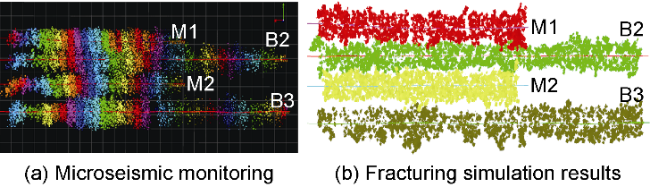
Fig. 2. Comparison between micro-seismic monitoring and fracturing simulation results of the Period 2 infill wells. (points of different colors represent fractures in different wells or intervals). |

Fig. 3. Validation of in-situ stress simulation results for period 2 infill wells. |
3. Inter-well interference mechanisms and fracturing parameters optimization
3.1. Inter-well interference mechanism of cube development infill well pad
3.1.1. Interference of fracture communication
Based on the established DFN-FEM hydraulic fracturing model and the actual fracturing parameters from each well's field operation, the fracture morphology of the X1 well pad was simulated. The fracture geometry parameters of infill wells in each infill period are listed in Table 2, and the fracture morphology is illustrated in Fig. 4.
Table 2. Statistics of fracture scale |
| Infill period | Well name | Fracture length/m | Fracture height/m | Width of SRV/m |
|---|---|---|---|---|
| Parent well | B1 | 201.34 | 27.27 | 137.52 |
| 1 | T1 | 139.56 | 19.70 | 115.33 |
| T2 | 140.81 | 21.34 | 116.01 | |
| 2 | B2 | 159.24 | 22.11 | 110.74 |
| B3 | 160.18 | 22.60 | 113.14 | |
| M1 | 155.77 | 15.80 | 101.47 | |
| M2 | 160.08 | 20.56 | 105.60 | |
| 3 | T3 | 141.10 | 19.90 | 115.65 |
| T4 | 140.75 | 20.98 | 114.50 |
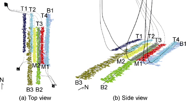
Fig. 4. Fracture morphology of cube development infill well pad (different colors represent fractures in different wells). |
In the early development stage, the hydraulic fracturing of the parent well B1 was aimed at fully stimulating the reservoir, thus resulting in a larger fracture scale. During infill Period 1, the infill well T1 and T2 in the top experienced no interference due to the large horizontal spacing from parent well B1 in the bottom, which had been producing for 6 years. For infill period 2, the fracturing design of infill wells M1/M2 in the middle and infill wells B2/B3 in the bottom required simultaneous consideration of interference from the parent well in the bottom reservoir and infill wells in the top. Specifically, Well M1 exhibited asymmetric fracture propagation due to stress shadow effects induced by the prolonged production history of Well B1, manifesting as significantly greater fracture extension in the east wing compared to the west wing. Additionally, due to the presence of a fracture zone between M1 and B1, fracturing fluid crossflowed toward B1’s fractures through the fracture zone, leading to significantly smaller fracture scale in well M1 (including fracture length, height and complexity) compared to well M2 (which was farther from B1). While Wells B2 and B3 experienced slight stress shadow, no obvious interference was observed in their fracture morphology due to their horizontal distance from Well B1 exceeding 360 m. In infill Period 3, due to the reservoir thickness of the top section being approximately equal to the sum of the middle and bottom sections, the infill wells T3 and T4 had a greater vertical distance from wells in the middle section, resulting in no inter-well interference. Meanwhile, it was also observed that the four infill wells in the top exhibited similar fracture geometry.
3.1.2. Interference of stress shadow
When infill wells are fractured at different times, variations in stress field conditions exist, which significantly affect the fracture propagation of infill wells. Fig. 5 shows the pore pressure, in-situ stress distribution, and horizontal stress difference in the target zone before infill well fracturing in each period. The pore pressure, minimum horizontal principal stress, and stress difference before the fracturing of parent well B1 were used as the initial values for the model. After Well B1 was put into production for 72 months, the infill Period 1 development was conducted. At this time, the pore pressure in the top section decreased by 10.0-20.5 MPa, the minimum horizontal principal stress had reduced by 9.0-12.5 MPa, and the stress difference had increased by 3.5-5.9 MPa. The stress disturbance range was 200 m, which did not affect the infill wells T1 and T2 in the top. During the infill Period 2, the infill wells T1 and T2 had a relatively short production time (7 months). The stress shadow did not affect the infill wells M1, M2 in the middle and the infill wells B2, B3 in the bottom. Due to the stress shadow caused by the long production of well B1, Wells M1 and B2 experienced stress interference. At this time, the pore pressure around well B1 had decreased by 10.0-30.5 MPa, the minimum horizontal principal stress had reduced by 15.0-20.5 MPa, the stress contrast had increased by 7.5-10.0 MPa, and the lateral stress disturbance range extended to 250 m. In the infill Period 3, Well M1 was influenced by the fracture zone and the production of Well B1. Well M1 exhibited a rapid pore pressure decline of 20.5 MPa within just 10 months of production, along with a 10.5 MPa reduction in minimum horizontal principal stress and a 3.8 MPa increase in stress difference. The magnitude of these stress changes was significantly greater than those observed in Wells T1 and T2 of infill Period 1. Analysis of stress distribution across the four infill periods reveals that stress evolution exhibits strong correlations with both the degree of reserve recovery by parent wells from reservoirs and the inter-well pressure communication. Stress evolution is the most dramatic during the first year of production, and then becomes more gradual over time.
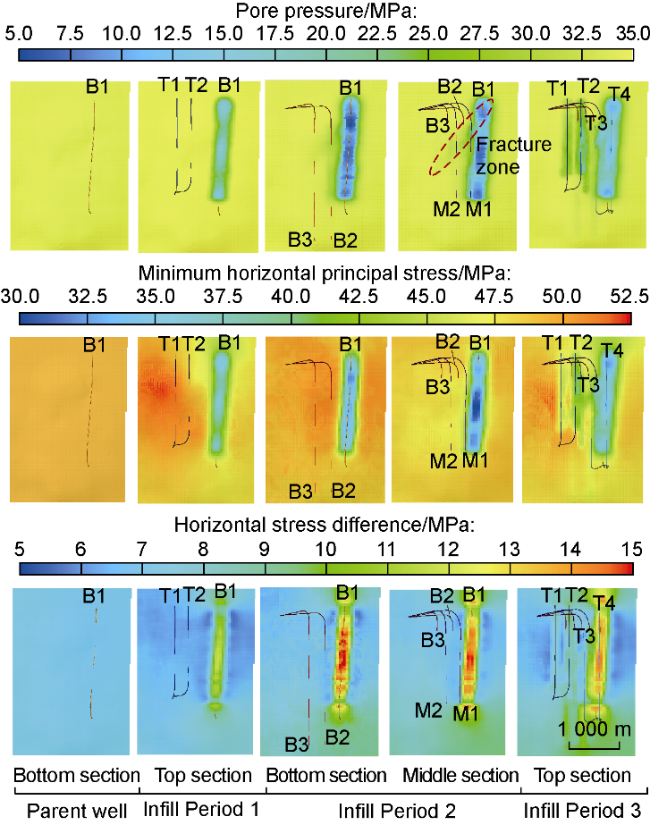
Fig. 5. In-situ stress evolution in different periods. |
3.1.3. Mechanism of inter-well interference in cube development infill well pad
Inter-well interference is influenced by multiple factors, which can be broadly categorized into geological and engineering factors: (1) Geological factors primarily include the development degree of natural fractures/faults, reservoir physical properties, geomechanical characteristics, and reservoir pressure distribution, etc. (2) Engineering factors mainly include well pattern and spacing, fracturing parameters (stage-cluster design, fluid volume, proppant volume, pumping rate, fracturing fluid properties, etc.), and production strategy, etc. The manifestation forms of inter-well interference can be classified by severity as follows: (1) The direct communication between hydraulic fractures in infill and parent wells results in frac-hit between wells. (2) Hydraulic fractures are connected through natural fractures or faults. (3) Pressure or stress disturbance. Considering the fracture and stress shadow interference in the X1 well pad, apart from the pressure communication between Well M1 in the middle and Well B1 in the bottom through natural fracture zones, and the stress shadow formed by B1, no other inter-well interference phenomena were identified in the simulation results. The inter-well interference in X1 well pad manifested as the latter two forms mentioned above.
From a mechanical mechanism perspective, the increase in stress difference around parent wells and the presence of fracture zones are the two primary reasons causing inter-well interference in this well pad. Long-term production and depletion in Well B1 have increased stress difference around the well, inducing hydraulic fractures of infill wells to propagate preferentially toward well B1. The intensity of this induced effect is closely related to both the degree of reserve recovery of Well B1 and the well spacing. In fracturing stages with developed nature fractures, hydraulic fractures tend to propagate along pre-existing natural fractures or faults, facilitating pressure communication between infill wells and parent wells through fracture zones. This results in rapid pressure decline in infill wells during the early production stage until pressure equilibrium is achieved with parent wells, negatively impacting the initial productivity and stable production performance of infill wells. The essence of the inter-well interference problem is the failure to properly handle the matching relationship among the well pattern, well spacing, and fracturing parameters. By setting reasonable infill well patterns, well spacing, and fracturing parameters, the probability of inter-well interference can be effectively reduced.
3.2. Optimization of fracturing parameters for cube development infill well pad
The X1 cube development infill well pad has a long development time span and complex well location relationships. This section took four infill wells of the infill Period 2 as an example for fracturing parameter optimization. The fracturing design for this period is particularly challenging due to the need to simultaneously consider interference from wells in both the top and bottom. The optimization process is based on the actual 3D geological model of X1 well pad. Using the average parameters of infill wells in same horizon as initial values, a controlled variable method is applied in the sequence of “well pattern/spacing-stage/cluster-fluid volume per stage”, focusing on two aspects: fracture geometry and productivity for parameter optimization.
3.2.1. Optimization of well pattern and well spacing
Reasonable deployment of infill well patternrepresents the most critical step to avoid inter-well interference. Closer well spacing will increase the probability of inter-well interference, whereas excessive spacing may leave unstimulated regions between adjacent wells. By altering well trajectories, two well patterns, rectangular and M-type, were devised (Fig. 6), where B1 is a parent well, B2, B3, M1, and M2 are infill wells.
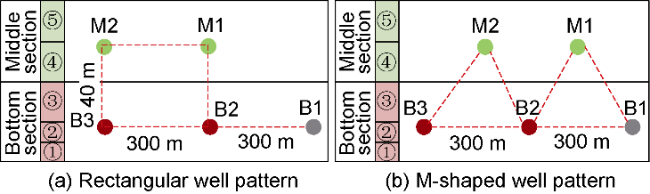
Fig. 6. Schematic diagrams of rectangular and M-shaped well patterns. |
Simulation results show that compared with the M-type well pattern, the rectangular well pattern exhibits significantly smaller SRV due to frac-hit in vertical, accompanied by a reduction in the number of activated natural fractures (Fig. 7a, 7b). The production forecasting of 5-year cumulative gas production is 1.3×10⁸ m3 lower than that of the M-type well pattern (Fig. 7c). In contrast, the M-shaped well pattern effectively mitigates inter-well interference risks while maximizing SRV, which demonstrates its applicability to cube development infill well pad.
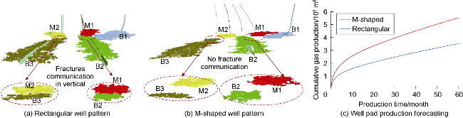
Fig. 7. Fracture communication and production forecasting for M-shaped and rectangular well patterns (points of different colors represent fractures of different wells in Fig. a and Fig. b). |
After the M-shaped well pattern was optimized, four different horizontal well spacings (350 m, 300 m, 250 m, and 200 m) were set to simulate fracture morphology, with results shown in Fig. 8. At a well spacing of 300 m, no inter-well interference occurred among the five wells (Fig. 8b), and fractures could propagate more freely when the spacing increased to 350 m. The cumulative gas production curves at 350 m and 300 m in Fig. 8a showed minimal difference and nearly overlapped, indicating that further increasing the spacing beyond 300 m had no significant impact on production. When the spacing was less than and equal to 250 m, the cumulative gas production curves shifted significantly downward, indicating frac-hit occurred as shown in Fig. 8c. Reducing the spacing further to 200 m caused the curves to decline more sharply, reflecting intensified pressure communication and frac-hit. Excessively small spacing induced inter-well fracture interference and pressure communication between parent and infill wells, which is the main reason for low productivity of infill wells. Balancing the objectives of productivity and maximum SRV, the optimal well spacing for the M-shaped well pattern was determined to be 300 m.
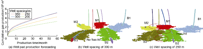
Fig. 8. Fracture communication and production forecasting for different well spacings (points of different colors represent fractures of different wells in Fig. b and Fig. c). |
3.2.2. Optimization of cluster spacing
Reasonable design of cluster spacing can improve the fracturing efficiency and achieve uniform reservoir stimulation. With the M-shaped well pattern and the well spacing of 300 m, keeping the fracturing stage length and the fluid volume per stage in Table 1 unchanged, four cluster spacings of 5, 10, 15, and 20 m were set for cluster spacing optimization simulation. It can be seen that as the cluster spacing decreases, the fracture length and the width of the SRV area show an obvious downward trend (Fig. 9), but the change in fracture height varies slightly. The production forecasting of the well pad shows (Fig. 10) that when the cluster spacing is 15 m and 20 m, although the fracture length is larger, the cumulative gas production of the well group is lower than that at a cluster spacing of 10 m. When the cluster spacing is 5 m, the cumulative gas production of the well group is the lowest, indicating that the optimal cluster spacing for the M-type well pattern is 10 m. “Dense cutting” hydraulic fracturing can avoid issues such as non-uniform fracture initiation and asymmetric propagation, increase fracture complexity and the activation of natural fractures, form high-conductivity complex fracture networks and enhance seepage efficiency. With the decrease in cluster spacing, the degree of asymmetric fracture propagation weakens. When the cluster spacing is reduced to 10 m, fracture propagation in each well becomes more balanced. When the cluster spacing is further reduced to 5 m, fractures only propagate in the near-wellbore area, with hindered outward propagation and insufficient extension, leading to a decrease in SRV (Fig. 11). Taking Well B2 as an example, when the cluster spacing is 15 m, the number of non-uniform propagation fracturing stages is 5. When the cluster spacing is reduced to 10 m, the non-uniform propagation fracturing stages decrease to 0. Therefore, when the fracturing stage length remains unchanged, a cluster spacing of 10 m is optimal.
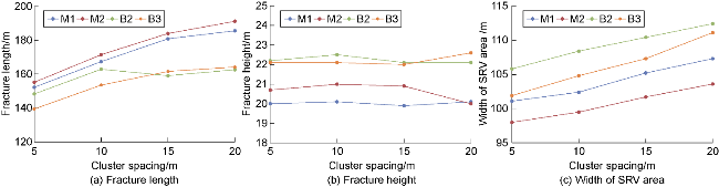
Fig. 9. Statistics of fracture scale under different cluster spacing. |
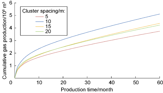
Fig. 10. Well pad production forecasting under different cluster spacings. |
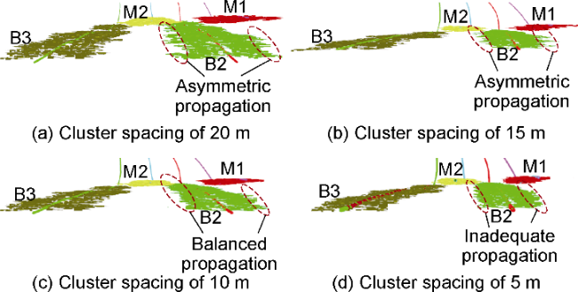
Fig. 11. Fracture communication under different cluster spacings (Points of different colors in the figure represent fractures in different wells). |
3.2.3. Optimization of fluid volume per stage
The fracturing fluid volume optimization simulation employed an M-shaped well pattern with 300 m well spacing and 10 m cluster spacing at fluid volumes per stage of 1 400, 1 600, 1 800, and 2 000 m3. The production forecasting results shows that when the fluid volume per stage reaches 1 800 m3, the effect of further increasing the fluid volume on production increment weakens (Fig. 12). Fracture geometry demonstrates that within the designed fluid volume range per stage, no fracture interference occurs. When the fluid volume increases from 1 400 m3 to 1 800 m3, the fracture geometry shows significant growth. However, as the volume further rises to 2 000 m3, the growth rate of fracture geometry slows (Fig. 13). Statistical results of fracture geometry under different fluid volumes indicate that fracture length and height, and width of SRV area all increase with fluid volume per stage (Fig. 14), but the growth rate slows down after the fluid volume exceeds 1 800 m3. When the fluid volume increases from 1 600 m3 to 1 800 m3, the fracture length, width of SRV area, and fracture height increase by 5.48%, 6.75%, and 4.39%, respectively. However, when the fluid volume per stage further increases from 1 800 m3 to 2 000 m3, the growth rates significantly decrease to 0.72%, 1.70%, and 0.76%. After comprehensive consideration of fracturing costs and production enhancement effects, the optimal fluid volume per stage is determined to be 1 800 m3.
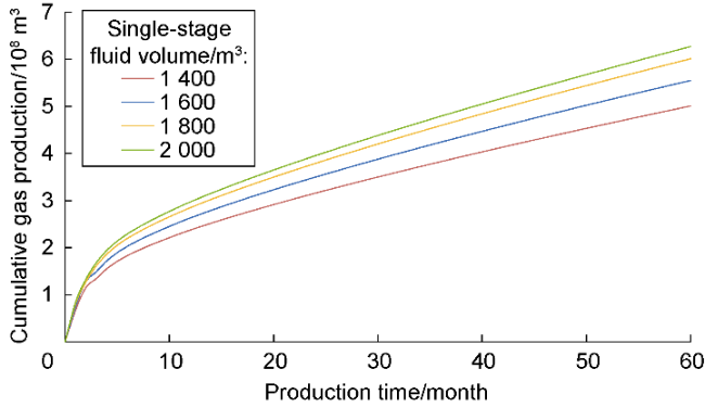
Fig. 12. Production forecasting of well pad after fracturing with different fluid volumes. |
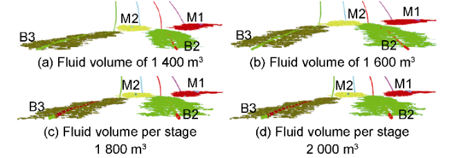
Fig. 13. Fracture communication under different fluid volumes per stage (Points of different colors in the figure represent fractures in different wells). |
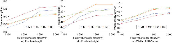
Fig. 14. Statistics of fracture scale under different fluid volumes. |
4. Application examples
4.1. Inter-well interference and the pressure recovery of parent wells
During the simulation of X1 well pad, it was observed that after the fracturing of Well M1 in the middle section, a fracture zone spanning the entire well group was activated. Pressure communication developed between Well M1 and Well B1, resulting in an approximately 10 MPa increase in pore pressure at Well B1 (Fig. 15). Monitoring data showed a significant wellhead pressure rise of well B1 (Fig. 16), confirming the high reliability of the simulation results.
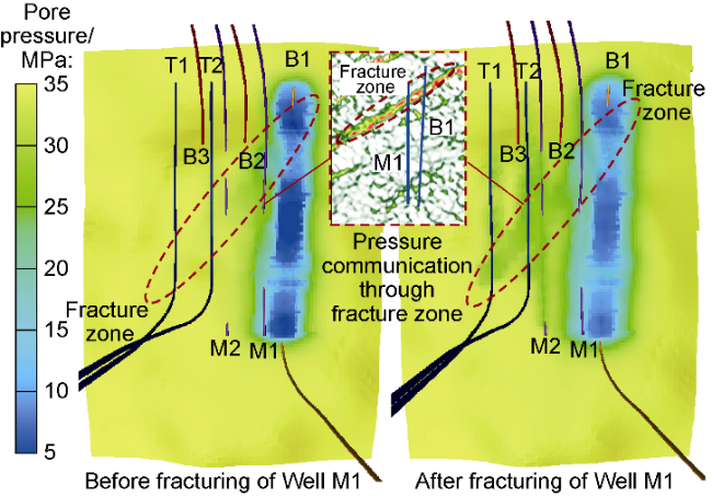
Fig. 15. Changes in pore pressure before and after fracturing of Well M1. |
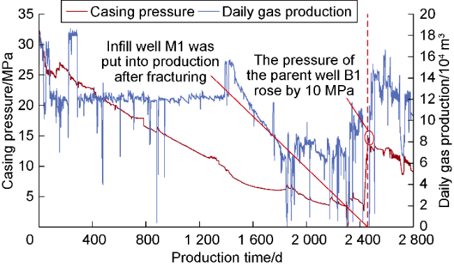
Fig. 16. Wellhead pressure and daily gas production curve of Well B1. |
Production monitoring data shows that after pressure communication was established between Well B1 and infill well M1, the daily gas production of Well B1 increased significantly (Fig. 16), and remained at a high level of 13×104 m3/d within 6 months after M1 was put into production. Compared with infill well M2 in the same layer and same infill period, although the startup pressure of Well M1 was 7 MPa lower, either of them can achieve the planned production target of 6.0×10⁴ m3/d within 1.5 years. This indicates that in the early stage of pressure communication, a synergistic effect occurs between the pressure recovery of parent well and the productivity release of infill well: parent well can enhance productivity through pressure recovery, while the early-stage productivity of infill well is not seriously affected. However, the two infill wells exhibited significant differences in long-term stable production performance. Well M2 maintained a daily gas production of (4.0-6.0)× 104 m3/d after 1.5 years of production. However, the daily production of Well M1 showed a stepwise decline with current daily production reduced to 2.0×10⁴ m3/d, which is basically the same as that of the parent well B1. This reflects that the inter-well pressure communication has have a delayed negative impact on the long-term sustained production of both infill wells and parent wells. This phenomenon is consistent with the infill well production experience in the Bakken and Haynesville Oilfields in North America. In the initial stage, about 1/3 of the inter-well interference can increase the productivity of parent well, which lasts for several months to one year. However, with the increase of production time, most of the inter-well interference will have a negative impact on the productivity of infill well and parent well [29-34].
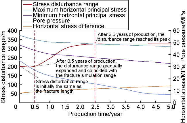
4.2. Characteristics of the influence range of in-situ stress evolution
Clarifying the evolution and disturbance range of in-situ stress is crucial for determining whether the fracture propagation of infill well is affected by stress interference from parent wells. Fig. 17 illustrates the variation curves of pore pressure, in-situ stress, and stress propagation range with time for Well B1 in the X1 well group. As can be seen from the figure: (1) The trend of in-situ stress change is basically consistent with the downward trend of pore pressure, with a rapid decline in the early stage of production. However, the decline rate of the maximum horizontal principal stress is lower than that of the minimum horizontal principal stress, leading to a continuous increase in the horizontal stress difference. (2) In the early stage of production, the lateral stress disturbance range is consistent with the fracture stimulation range (the fracture stimulation range of Well B1 is shown in Table 2). After 0.5 years of production, the disturbance range gradually expands, and reaches its peak after 2.5 years. At this time, the disturbance range is about 1.5-1.6 times the length of the fracture.
Fig. 17. In-situ stress and pore pressure disturbance curve of Well B1. |
4.3. Field application results
The parameter optimization method for infill well fracturing proposed in this paper was applied to design the infill well fracturing plan for X1 well pad, successfully mitigating the risk of inter-well interference caused by close spatial distances during three-layer cube development. In the second infill period, 4 infill wells were drilled, achieving a combined initial gas production rate of 67×104 m3/d (averaging 16.75×10⁴ m3/d per well). As of the middle of May 2025, the four infill wells have been in production for over 1 590 d. Currently, the wellhead pressure of the four wells remains at 2.8-4.4 MPa, with an average daily production of (4.8-6.1)×104 m3, demonstrating stable production performance (Table 3). Through cube development, the well group recovery factor increased to 44.3%, 30 percentage points higher than the block average, significantly improving reserve utilization. The first-year production decline rate decreased by nearly 10 percentage points compared to the block average, demonstrating favorable development results.
Table 3. Production data of infill wells |
| Well | Production duration/d | Wellhead pressure/MPa | Current daily gas production/104 m3 | Average daily gas production/104 m3 | Cumulative gas production/104 m3 | |
|---|---|---|---|---|---|---|
| Startup | Current | |||||
| M1 | 1 593 | 16.8 | 2.8 | 2.0 | 4.8 | 6779.8 |
| M2 | 1 593 | 23.8 | 3.5 | 4.5 | 5.5 | 8294.0 |
| B2 | 1 590 | 24.2 | 4.3 | 3.8 | 5.7 | 8211.5 |
| B3 | 1 590 | 23.4 | 4.4 | 3.8 | 6.1 | 8778.6 |
5. Conclusions
After the X1 infill well pad was put into production, the trend of in-situ stress evolution was basically consistent with the downward trend of pore pressure in the early stage of production. As the production time increased, the horizontal stress difference continuously increased. After 0.5 years of production, the lateral disturbance range began to gradually expand and reached its peak after 2.5 years, with the peak value being approximately 1.5-1.6 times the fracture length.
The increase in the horizontal stress difference and the presence of fracture zone are the main reasons for inter-well interference. Inter-well interference is likely to occur near the fracture zone and between the infill wells and the parent wells with a long production time. The key to avoiding inter-well interference is to optimize the fracturing parameters. As for the M-shaped well pattern, the optimal well spacing of the infill wells is 300 m, the cluster spacing is 10 m, and the fluid volume per stage is 1800 m3.
The pressure communication between infill wells and parent wells can generate synergistic effects in the short term, manifesting as productivity recovery of parent well and the productivity release of infill well, thereby improving the productivity of parent well. However, from a long-term production sustainability perspective, inter-well interference exerts delayed negative impacts on the productivity of both infill wells and parent wells.
Nomenclature
C—fracture cohesion, Pa;
Cf,i—three-dimensional fracture compressibility coefficient, Pa-1;
Cf0,i—initial fracture compressibility coefficient, Pa-1;
Cg—total gas compressibility coefficient, Pa-1;
d—fracture propagation distance, m;
dmax—maximum fracture propagation distance, m;
D—relative elevation, m;
Dk—Knudsen diffusion coefficient, m2/s;
e(u)—strain tensor (representing shear strain), dimensionless;
E—elastic modulus, Pa;
Ei—three-dimensional elastic modulus, Pa;
f(σ)—effective stress normal to fracture plane, Pa;
g—gravitational acceleration, m/s2;
H—fracture height, m;
I—second-order unit tensor, dimensionless;
i—stress/strain direction (1-3, where 1 and 3 represent horizontal principal stresses, 2 represents vertical);
Keff—apparent permeability, m2;
Kf—natural fracture permeability, m2;
KF—main hydraulic fracture permeability, m2;
KF0—initial main hydraulic fracture permeability, m2;
KFi—three-dimensional permeability, m2;
Krgf—gas relative permeability in fractures, dimensionless;
Krwf—water relative permeability in fractures, dimensionless;
p—current pore pressure, Pa;
p0—initial pore pressure, Pa;
pf—pressure in natural fractures, Pa;
pF—pressure in main hydraulic fractures, Pa;
pgf—gas pressure in fractures, Pa;
pm—matrix pore pressure, Pa;
pfrac—fluid pressure in fractures, Pa;
ppu—pumping pressure, Pa;
pwf—water pressure in fractures, Pa;
qmtc—gas mass flow rate in matrix, kg/(m3·s);
qw—water mass flow rate, kg/(m3·s);
qg—gas mass flow rate, kg/(m3·s);
s—leak-off coefficient, 0-1, dimensionless;
Sgf—gas saturation in natural fractures, %;
Swf—water saturation in natural fractures, %;
t—time, s;
u—displacement, m;
vf—gas flow velocity in natural fractures, m/s;
vF—gas flow velocity in main hydraulic fractures, m/s;
vkm—gas diffusion velocity, m/s;
vm—gas seepage velocity in matrix, m/s;
vs—slippage velocity, m/s;
VF—fracturing fluid volume in fractures, m3;
VI—injected fracturing fluid volume, m3;
VL—leaked-off fluid volume, m3;
W—hydraulic fracture width, m;
x—coordinate along fracture length, m;
y—coordinate along fracture width, m;
α—Biot coefficient, dimensionless;
βi—three-dimensional variation rate of fracture compressibility coefficient, Pa-1;
·u—divergence of displacement (representing normal strain), dimensionless;
υ—Poisson’s ratio, dimensionless;
υi—three-dimensional Poisson’s ratio, dimensionless;
ρg—gas density, kg/m3;
ρL—fracturing fluid density, kg/m3;
ρw—water density, kg/m3;
θ—internal friction angle, (°);
μg—gas viscosity, Pa•s;
μw—water phase viscosity, Pa•s;
ϕf—natural fracture porosity, %;
ϕF—hydraulic fracture porosity, %;
ϕF0—initial hydraulic fracture porosity, %;
ϕm—matrix porosity, %;
σe,i—three-dimensional effective stress, Pa;
σe0,i—three-dimensional initial effective stress, Pa;
Δσe,i—three-dimensional effective stress variation Pa;
σ—total stress, Pa;
σ'—effective stress, Pa;
σN—fracture normal stress, Pa;
σw—circumferential tensile stress, Pa;
σT—tensile strength, Pa;
τ—shear strength, Pa.