

Introduction
Hydraulic fracturing, as a pivotal technology for developing unconventional oil and gas resources, fundamentally relies on constructing an artificial fracture network within the reservoir through high-pressure fluid injection. By leveraging the suspension transport capability and high compressive strength of proppants (e.g. quartz sand, and ceramic particles) to maintain fracture flow, a “subsurface highway” system for oil and gas migration is formed, thereby ensuring the subsequent flow of oil and gas into the wellbore. The effective placement rate of proppants within the fracture network directly determines the effect of fracturing stimulation. Unraveling the transport and placement patterns of proppants within complex fracture networks holds significant en-gineering implications for improving the recovery factor of unconventional oil and gas reservoirs and optimizing hydraulic fracturing schemes [1-3].
During hydraulic fracturing of unconventional reservoirs, the transport of proppants exhibits multifactor coupling characteristics, and their spatial distribution is primarily controlled by three aspects: (1) the complex geometry and network structure of the fracture system, which determines the spatial heterogeneity of transport paths; (2) the thermo-fluid-solid coupling effect formed by fluid properties, temperature fields, and proppant characteristics, which dominates the transport dynamics; and (3) the compatibility between engineering parameters and the fracture network, which directly influences the placement effectiveness of proppants. Early research mostly focused on proppant transport within single fractures, observing sedimentation and distribution patterns experimentally, and establishing corresponding models based on mass-momentum equations. In recent years, research has gradually expanded to complex fracture networks, further incorporating fluid properties, temperature variations, and proppant attributes, making simulations more aligned with actual engineering conditions. Scholars have used acrylic glass to construct multi-level fracture physical simulation devices, studying the transport patterns of proppants in complex fracture networks, and analyzing the influence mechanisms of branch fractures on proppant transport. For instance, Sahai et al. [4] simulated proppant transport under 27 different operating conditions within geometrically complex fractures, finding that the pump injection rate is the main factor affecting proppant transport and sedimentation in complex fractures. Tong et al. [5] conducted experiments similar to Li et al. [6], studying the effects of branch fracture angles and proppant particle sizes on transport, observing that proppants with smaller particle sizes are more likely to enter branch fractures.
Physical experiments are limited by factors such as downsized devices, incomplete simulation of fracture morphology, and high experimental costs, making it difficult to fully replicate the real complex fracture networks. In contrast, numerical simulation technology can better describe the influence of fracture morphology, particle, and fluid properties on proppant transport, featuring high efficiency and low cost. Current numerical simulation methods for proppant transport in complex fracture networks are developing in multiple directions. Scholars have employed traditional computational fluid dynamics-discrete element method (CFD-DEM) and computational fluid dynamics-discrete phase model (CFD-DEM) fluid-solid coupling methods to simulate particle transport in T-shaped, cross, and branch fractures [7-9]. Gong et al. [10] successfully reproduced the bridging phenomenon in narrow fractures through CFD-DEM simulations, quantitatively revealing the critical bridging conditions. Ren et al. [11] established a liquid-solid two-phase flow model using CFD-DEM, discovering that low-density proppants are placed more uniformly in complex fractures, with weaker accumulation at fracture mouths. Zhou et al. [12] utilized the Lattice Boltzmann method (LBM) to simulate the impact of wall-retardation effect in rough fractures on proppant transport, finding that local narrow flow channels enhance wall-retardation effects, but the fracture shape no longer significantly influences the transport mode in rough fractures when the roughness height is much smaller than the fracture aperture. Patel et al. [13] established an Eulerian-Granular model to quantify the transport characteristics when the particle phase volume fraction is 45%-50% under low-temperature environments. Yang et al. [14] employed a three- dimensional discontinuous displacement Euler-Euler model to achieve coupled simulation of fracture network expansion and proppant transport at the well scale, but the methodology was limited for not considering particle-scale dynamics, making it difficult to capture microscopic mechanisms such as proppant bridging, sedimentation, and blockage. In summary, existing methods still face multiple constraints in simulation scale, computational accuracy, and cost, so they cannot simultaneously meet the engineering needs for field-scale fracture networks and low-cost simulations.
This study employs a three-dimensional multi-phase particle-in-cell (MP-PIC) method, together with an Eulerian-Lagrangian hybrid solver for field-scale simulations. The continuous phase fluid motion is described by the Navier-Stokes equations, the discrete particle phase is tracked in a Lagrangian framework to resolve individual particle dynamics, and a two-way momentum exchange term accurately captures the fluid-solid coupling effects [15]. Algorithmically, the concept of a virtual particle cluster is introduced. Through a multi-scale coupling strategy that integrates microscopic collision statistics with macroscopic pressure gradients, the computational complexity of high-concentration particle systems is reduced by two orders of magnitude. Based on this, a complex fracture network model is constructed. Under varying parameter conditions, the distribution patterns and influence ranges of proppants within the fractures are analyzed. The study clarifies the transport mechanisms and patterns of proppants in complex fracture networks, aiming to provide technical support for field fracturing design.
1. Theoretical model
The MP-PIC method is a numerical simulation technique based on the Eulerian-Lagrangian approach. Its core principle lies in treating fluids as discrete mass points, wherein the flow dynamics are collectively governed by the conservation equations of mass, momentum, and energy. Particles are simultaneously considered as individual entities and as continuums. In dense flows, calculating the stress gradient for each particle is challenging; thus, it can be approximated as a gradient on the computational grid and subsequently interpolated onto the discrete particles. This treatment enables a balance between capturing physical details and computational efficiency in large-scale industrial particle systems [16-20].
1.1. Continuous phase governing equations
Based on the MP-PIC method for liquid-solid two-phase simulation, considering that there is no mass transfer between the liquid and solid phases, the fluid phase is incompressible, and the fluid phase and the particle phase are at the same temperature, the continuity equation for the fluid can be expressed as:
Considering the presence of a dense solid phase, there exists an interaction between the fluid and the proppant. By introducing the volume fraction and the fluid-particle interaction term to account for the coupling effect of the solid phase, the momentum equation for the fluid can be expressed as:
The non-hydrostatic part of the stress depends solely on the strain rate component Sij, as expressed by the following equation:
For a Newtonian fluid, the stress is:
Considering the relatively high flow velocity near the fracture aperture, the large eddy simulation (LES) model [21] is introduced on the basis of the continuous phase governing equation to characterize the turbulent features of fracturing fluid under high Reynolds numbers. The key of the model is to introduce spatial filtering operations, defining ‘~’ as the spatial filtering function, with the filtering scale taken as the grid size. The filtered continuity equation and momentum equation are as follows:
$ \begin{array}{c} \frac{\partial\left(\rho_{\mathrm{f}} \tilde{\alpha}_{\mathrm{f}} \tilde{\boldsymbol{u}}_{\mathrm{f}}\right)}{\partial t}+\nabla \cdot\left(\rho_{\mathrm{f}} \tilde{\alpha}_{\mathrm{f}} \tilde{\boldsymbol{u}}_{\mathrm{f}} \tilde{\boldsymbol{u}}_{\mathrm{f}}\right)=-\alpha_{\mathrm{f}} \nabla \tilde{p}- \\ \boldsymbol{\beta}_{\mathrm{fp}}-\alpha_{\mathrm{f}} \nabla \cdot\left(\tilde{\boldsymbol{\tau}}_{\mathrm{f}}+\tilde{\boldsymbol{\tau}}_{\mathrm{f}, \mathrm{SGS}}\right)+\rho_{\mathrm{f}} \alpha_{\mathrm{f}} \boldsymbol{g} \end{array}$
In Eq. (6), and represent the filtered stress tensor and the sub-grid scale (SGS) stress tensor, respectively. The filtered stress tensor is calculated by:
where, and are calculated by:
1.2. Particle phase control equation
It is assumed that the mass of particles remains constant over time (that is, there is no mass transfer between particles or between particles and fluid), but particles have different sizes and densities. The evolution of the particle distribution function ϕ over time is obtained by solving the Liouville equation [22], and Eq. (11) is a generalized form of the Boltzmann equation that describes the conservation of particle numbers in the volume elements moving along the kinetic trajectories in space.
In the numerical program, Eq. (11) is not solved directly. Instead, the particle phase is treated as discrete computational particles. Each computational particle represents a group of particles that have the same density, volume, velocity, and specific position. Their motion follows the Newton’s second law:
The distinctive feature of this acceleration model lies in its integration of the pressure gradient concept from continuum mechanics with the particle interaction principles of DEM, thereby establishing a unique hybrid modeling framework.
Based on Eq. (11), the macroscopic conservation equation is derived. By applying the divergence theorem and considering the boundary conditions, the integral of the divergence term in velocity space becomes zero, leading to the continuity equation for the particle phase:
By multiplying Eq. (11) by , integrating over the density, volume, and velocity spaces, and subsequently performing vector operations, the momentum equation for the particle phase is derived.
$ \begin{array}{l} \frac{\partial\left(\alpha_{\mathrm{p}} \rho_{\mathrm{p}} \boldsymbol{u}_{\mathrm{p}}\right)}{\partial t}+\nabla \cdot\left(\alpha_{\mathrm{p}} \rho_{\mathrm{p}} \boldsymbol{u}_{\mathrm{p}} \boldsymbol{u}_{\mathrm{p}}\right)=-\alpha_{\mathrm{p}} \nabla p-\nabla \tau_{\mathrm{p}}+ \\ \alpha_{\mathrm{p}} \rho_{\mathrm{p}} \boldsymbol{g}+\iiint \phi \Omega_{\mathrm{p}} \rho_{\mathrm{p}} D_{\mathrm{p}}\left(\boldsymbol{u}_{\mathrm{f}}-\boldsymbol{u}_{\mathrm{p}}\right) \mathrm{d} \Omega_{\mathrm{p}} \mathrm{~d} \rho_{\mathrm{p}} \mathrm{~d} \boldsymbol{u}_{\mathrm{p}}- \\ \nabla \cdot\left[\iiint \phi \Omega_{\mathrm{p}} \rho_{\mathrm{p}}\left(\boldsymbol{u}_{\mathrm{p}}-\overline{\boldsymbol{u}}_{\mathrm{p}}\right)\left(\boldsymbol{u}_{\mathrm{p}}-\overline{\boldsymbol{u}}_{\mathrm{p}}\right) \mathrm{d} \Omega_{\mathrm{p}} \mathrm{~d} \rho_{\mathrm{p}} \mathrm{~d} \boldsymbol{u}_{\mathrm{p}}\right] \end{array}$
1.3. Interfacial force equation
In solid-liquid two-phase flow, solid particles are influenced by multiple liquid forces, including drag force, buoyancy, and Saffman lift. Considering computational performance, for purpose of efficiency, only the primary forces (buoyancy and drag force) are considered here. The buoyancy exerted on particles during the flow of the proppant-fracturing fluid mixture is expressed as:
$F_{\mathrm{f}}=-\frac{\pi}{6} d_{\mathrm{p}}^{3} \rho_{\mathrm{f}} \boldsymbol{g}$
Based on the model proposed by Filippo et al. [23], Gidaspow introduced a drag model that accommodates both dilute and dense particle systems [24]. This model describes the interphase momentum exchange rate arising from the velocity difference between the liquid and solid phases using the drag coefficient (λd), and it is calculated by:
where, the dimensionless drag coefficient (λd) is a dimensionless term, and it is expressed as:
1.4. Interpolation operator
In the MP-PIC method, the interpolation operator is a crucial mathematical tool that bridges the Eulerian description of the fluid phase and the Lagrangian description of the particle phase [25]. This coupling is essential due to the nature of the physical problem: the fluid phase is best described using the Eulerian approach of continuum mechanics, while the trajectories of discrete particles naturally align with Lagrangian tracking. The interpolation operator facilitates two-phase coupling through bidirectional mapping: mapping discrete particle attributes (e.g. volume and momentum) onto the Eulerian grid, and mapping grid-computed field variables (e.g, pressure gradients and stresses) back to the particle positions.
The linear interpolation operator used in this study is constructed as the product of directional operators in the x, y, and z directions.
The bidirectional mapping between particle attributes and the Eulerian grid is achieved through trilinear interpolation. This interpolation operator can be decomposed into the product of three orthogonal one-dimensional operators (e.g., along the x, y, and z axes). For a particle located at wp = (xp, yp, zp), the component of the grid cell I interpolation operator in the x-direction is an even function, independent of the y and z coordinates, and possesses the following properties.
The linear interpolation operator for a cell along the x-direction is defined on the computational grid as:
In the context of computational grids, the particle volume fraction at cell k resulting from the mapping of particle volumes is expressed as:
According to the principle of volume conservation, the sum of the fluid and particle volume fractions equals 1, i.e., .
When coupling the governing equations, the interphase momentum exchange term βfp in the fluid momentum equation (Eq. (2)) can be discretized via the interpolation operator as follows:
where, Ok serves as the interpolation operator that maps particle attributes to grid node k. The particle drag force and attributes are mapped to the Eulerian grid nodes via the interpolation function. If a top-hat interpolation is employed, the fluid velocity at the particle position wp depends solely on the velocity value at a single node. Conversely, if trilinear interpolation or other higher-order methods are used, the fluid velocity is obtained through a weighted average of multiple node velocities, facilitating a smoother transmission of field variables.
The particle collisions are characterized by the particle normal stress. This stress is derived from the particle volume fraction, which, in turn, is calculated based on the particle volume mapped onto the grid. The model for particle normal stress is expressed as [26]:
In the particle acceleration equation (Eq. (12)), except for gravity, all force-related terms need to be obtained from the grid through interpolation, which is achieved by the following equation:
$Q_{\mathrm{p} k}=\sum_{l=1}^{N_{\mathrm{p} k}} O_{k}\left(x_{\mathrm{p}}\right) Q_{k l}$
Essentially in the MP-PIC method, a fully implicit coupling is achieved. This approach links the discretized particle motion equations with the discretized fluid momentum equations through interpolation operators, constructing a unified linear system of equations.
2. Model verification
Based on the proppant transport and sedimentation experiments conducted by Zhang et al. [27], a proppant transport model for branch fractures of identical dimensions was established. The specific parameters are as follows: the main fracture measures 400 cm in length, 30 cm in height, and 1 cm in width; the branch fracture measures 100 cm in length, 30 cm in height, and 1 cm in width; the angle between the main fracture and the branch fracture is 30°. In the model, three circular injection inlets with a diameter of 10 mm are uniformly distributed at the entrance of the main fracture. The fracturing fluid, carrying proppant, is pumped through the circular injection inlets into a vertical slot to complete the transport and placement of the proppant. The model input parameters remain consistent with those in Reference [27] (Table 1), and the physical model is illustrated in Fig. 1.
Table 1. Main input parameters for physical experiments and simulations |
| Parameter | Value | Parameter | Value |
|---|---|---|---|
| Fracture width | 1.0 cm | Proppant density | 2 650 kg/m3 |
| Fracture height | 30 cm | Fluid density | 997 kg/m3 |
| Main fracture length | 400 cm | Fluid viscosity | 2.3 mPa·s |
| Branch fracture length | 100 cm | Injection rate | 1.67 m/s |
| Proppant particle size | 0.3 mm |
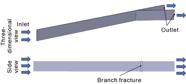
Fig. 1. Vertical fracture proppant transport numerical model. |
Comparing the experimental and numerical simulation results of the sand dike height inside the fracture (Fig. 2), it can be observed that with the continuous injection of proppants, the sand dike height inside both the main and branch fractures continuously increases. At 140 s, the sand dike height in the main fracture increases with distance from the injection inlet, reaching a maximum near the entrance of the branch fracture, approximately 0.28 m. Conversely, in the branch fracture, the sand dike height decreases with distance from the entrance, dropping rapidly near the outlet. The comparison shows a good consistency between simulation and experimental results. At 70 s, the errors of numerical simulation results relative to experimental results in sand dike height for the main and branch fractures are 7.7% and 8.4%, respectively. At 140 s, the errors of numerical simulation results relative to experimental results are 8.9% and 7.8%, respectively. Further comparison of the relationship curves between proppant transport distance and sand dike height under different injection times (Fig. 3) shows that the overall trends of experimental and simulation data are very similar, with average simulation errors of 7.8% for the main fracture and 7.0% for the branch fracture. These results indicate that the model established in this paper is reliable, and the simulation accuracy generally meets the engineering design requirements.
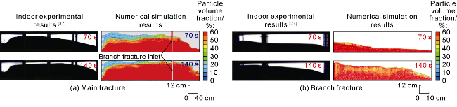
Fig. 2. Comparison of sand dike height between indoor experiments and numerical simulations. |
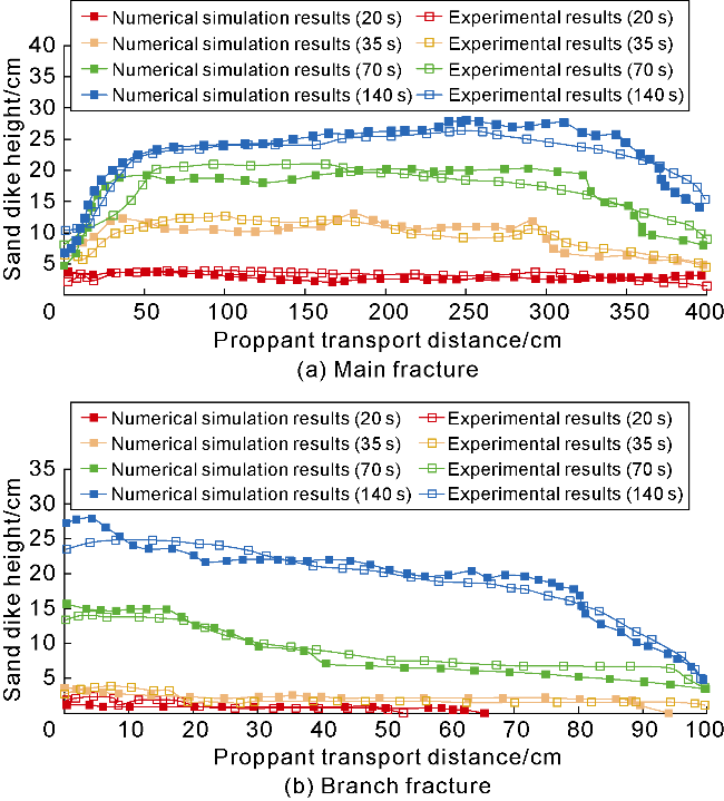
Fig. 3. Relationship between proppant transport distance and sand dike height under varying injection times. |
3. Results and discussion
The sand dike equilibrium height is a conventional metric for evaluating the vertical placement efficiency of proppants; however, it falls short in assessing the planar distribution of proppants. Consequently, this study introduces the proppant planar placement coefficient, which is defined as the ratio of the area affected by the proppant to the controlled area of the fracture network physical model.
3.1. Model construction
Fig. 4 depicts the constructed fracture network model. The main fracture extends along the x‑axis, featuring a height of 5 m, a length of 60 m, and an aperture of 8 mm. The branch fractures extend along the y‑axis, each with a length of 40 m and an aperture of 2 mm. Balancing computational efficiency with simulation accuracy, the model is discretized using hexahedral elements, resulting in a total of 2 338 256 cells. A constant pressure boundary condition is applied at the right end of the main fracture and at the outlets of each branch fracture. The parameters for the proppant and fracturing fluid are listed in Table 2.
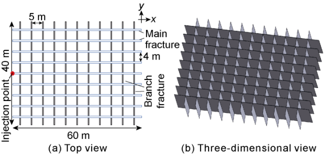
Fig. 4. Schematic diagram of the fracture network model. |
Table 2. Simulation parameters |
| Parameter | Value | Parameter | Value |
|---|---|---|---|
| Proppant density | 1 200-2 400 kg/m3 | Inlet flow rate | 0.5-2.0 m3/min |
| Proppant particle size | 0.2-0.8 mm | Boundary pressure | 37 MPa |
| Fracturing fluid density | 1 000 kg/m3 | Proppant volume ratio | 8% |
| Fracturing fluid viscosity | 1-15 mPa·s | Fracture included angle | 90° |
3.2. Proppant transport in complex fracture networks
Based on the parameters in Table 2 and a fixed injection rate of 0.4 m3/min, the evolution of proppant transport within the complex fracture network was simulated (Fig. 5). The transport process can be delineated into three distinct stages:
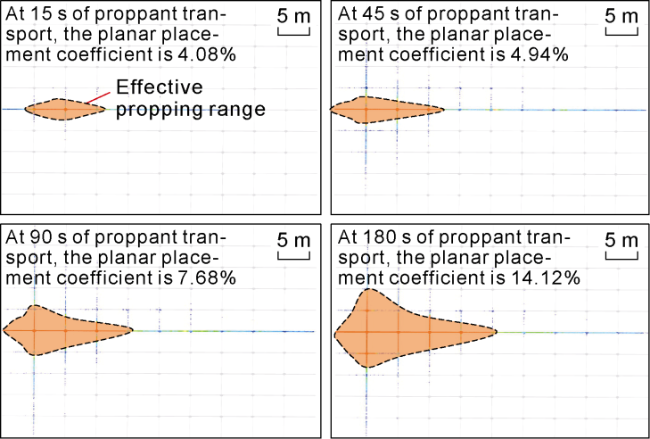
Fig. 5. Variation in planar placement efficiency of proppants (top view). |
(1) Initial filling stage (0-15 s): Proppants rapidly deposit near the wellbore within the main fracture, forming a high-concentration accumulation zone. The effective propping region appear a droplet-like morphology, with a planar placement coefficient of 4.08%.
(2) Dominant channel formation stage (15-45 s): Proppants migrate further downstream within the main fracture, with a portion entering branch fractures to form localized sand dike. Along the main fracture, the effective propping length continuously increases, and the planar placement coefficient rises to 4.94%.
(3) Fracture network extension stage (45-180 s): The sand dike within the main fracture reaches an equilibrium height near the wellbore, leading to increased flow resistance. Under the combined influence of fracturing fluid drag and sand dike resistance, proppants flow into branch fractures. Both the main and branch fractures exhibit continued growth in effective propping length, with the planar placement coefficient reaching 14.12%. It is noteworthy that the growth rate of effective propping length along the main fracture significantly exceeds that of the branch fractures. This discrepancy is attributed to the differential flow resistance gradients between main and branch fractures, where inertial effects preferentially drive particle migration along the main fracture, thereby establishing a dominant channel effect that constrains proppant transport within the branch fractures.
The fluid flow patterns during proppant transport were examined (Fig. 6). In the initial filling stage, the fluid streamlines exhibit a multi-directional vortex structure. This primarily originates from the mechanism that the high-pressure fluid (Re > 2 300) entering the fracture collides with the fracture walls, inducing the turbulent dissipation, which in turn generates local eddies. During this stage, the trajectories of proppant particles are highly irregular due to the influence of these vortices. Although a small fraction of particles diffuse downstream via the vortex flow, the majority of the proppant forms a temporary accumulation near the wellbore. This is due to the combined hindrance of high-frequency inter-particle collisions and wall friction, resulting in a non-uniform, patchy distribution of proppant. In the dominant channel formation stage, as the sand dike height continues to increase, the flow passage between the fracture roof and the top of the sand dike narrows. This leads to an acceleration of the fracturing fluid and proppant flow velocities, and the formation of vortices at the top of the sand dike, which smoothens the dike surface. Simultaneously, the fluid streamlines evolve from an initial chaotic state to 3-4 main conduits, allowing the particle ensemble to achieve a stable transport state through dissipative dynamics. Owing to the significantly higher pressure drop gradient in the main fracture compared to the branch fractures, the fluid preferentially follows the low-resistance path, ultimately establishing a stable dominant transport channel. In the fracture network extension stage, a substantial amount of proppant accumulates near the wellbore. As the fracturing energy is affected by viscous dissipation within the sand dike, the Reynolds number begins to reduce, and the streamlines tend to be parallel. Concurrently, the reduction in fluid velocity within the main fracture diminishes its channel advantage, prompting the fluid carrying the proppant to redirect into secondary fractures. This redirection significantly enhances the planar placement coefficient of the proppant. In summary, the fluid flow regime during the fracturing fluid injection process transitions sequentially from vortex-dominated flow to transitional flow, and finally to laminar flow.
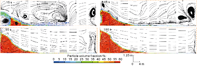
Fig. 6. Fluid flow regime distribution during proppant transport (side view). |
3.3. Transport characteristics of proppants in complex fracture networks
Based on the simulation parameters in Table 2, a model was established with an injection duration of 390 s. Throughout the simulation, the fundamental model parameters were held constant, and only a single parameter was varied at a time to investigate the influence of proppant density, proppant particle size, fracturing fluid viscosity, and the angle between main and branch fractures on proppant placement performance.
3.3.1. Impact of proppant density
In this study, the proppant density was varied to 1 200, 1 600, 2 000, and 2 400 kg/m3 to simulate the effect of proppant density on placement efficiency. It is found that the higher the proppant density, the greater the density difference between the proppant and the fracturing fluid, resulting in a higher gravitational settling rate. Consequently, proppants tend to settle rapidly at the near-wellbore region, forming a concentrated and thick sand dike. This shortens the proppant transport distance and thins the distal sand dike (Fig. 7). As the proppant density increases, the planar placement coefficient of the proppant gradually decreases (Fig. 8). When the proppant density is 2 400 kg/m3, the planar placement coefficient is 13.78%, whereas at a density of 1 200 kg/m3, the coefficient is 25.45%, reflecting an increase of 11.67 percentage points. In summary, sand-carrying fluids have limited suspension and transport capabilities for high-density proppants, making them ineffective for long-distance transport. Therefore, low-density proppants are recommended for expanding the treatment area, while high-density proppants are advisable for enhancing near-wellbore flow capacity.
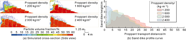
Fig. 7. Effect of proppant density on the morphology of the main fracture sand dike. |
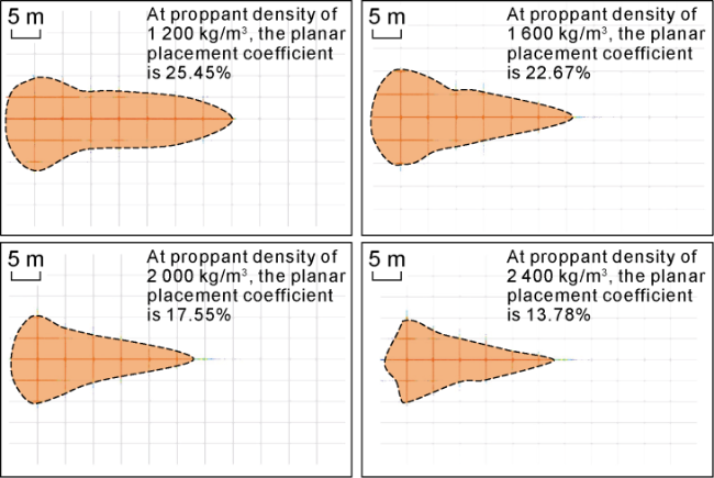
Fig. 8. Effect of proppant density on planar placement efficiency (top view). |
3.3.2. Impact of proppant particle size
The particle size of the proppant was varied to 0.2, 0.4, 0.6, and 0.8 mm to simulate the impact of proppant particle size on placement efficiency. According to the simulation results, when the proppant particle size is 0.2 mm, the transport distance reaches 40.78 m, effectively reaching the distal fracture. The resulting sand dike is uniformly distributed along the fracture length, and the placement morphology is relatively flat (Fig. 9). As the particle size increases from 0.2 mm to 0.8 mm, the slope angle of the sand dike front edge gradually decreases. Larger particles are more influenced by gravity, leading to faster settling. Consequently, they primarily accumulate at the near-wellbore region, forming a higher sand dike with a shorter placement distance, making it more difficult for the proppant to enter the branch fractures. The smaller the particle size, the larger the planar coverage area is. At a particle size of 0.2 mm, the planar placement coefficient reaches 29.70%. In contrast, larger particles settle more easily, limiting their transport distance and reducing their planar coverage area. At a particle size of 0.8 mm, the planar placement coefficient is only 17.45%, a decrease of 12.25 percentage points compared to the 0.2 mm scenario (Fig. 10). Therefore, low-particle-size proppants are recommended for expanding the treatment area at the distal end, while large-particle-size proppants are more suitable for enhancing the near-wellbore flow capacity.
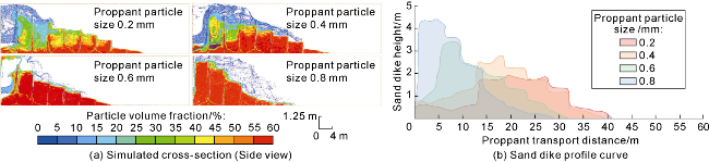
Fig. 9. Effect of proppant particle size on the morphology of the main fracture sand dike. |
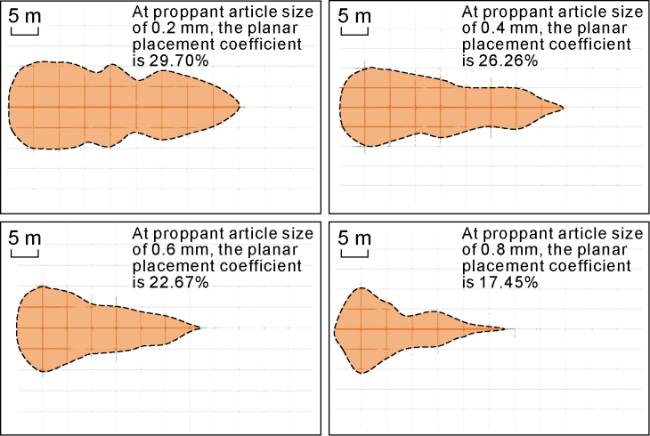
Fig. 10. Effect of proppant particle size on planar placement efficiency (top view). |
3.3.3. Impact of fracturing fluid viscosity
The viscosity of the fracturing fluid was varied to 1, 5, 10, and 15 mPa·s to simulate its impact on proppant placement efficiency. The simulation results reveal that the lower the viscosity of the fracturing fluid, the weaker its sand-carrying capacity, resulting in poorer proppant transport in the main fracture and a shorter transport distance. Therefore, at lower viscosities (e.g., 1 mPa·s), proppants primarily accumulate at the near-wellbore end, forming a higher sand dike that provides effective support for the near-wellbore fractures. Conversely, as the viscosity of the fracturing fluid increases, its sand-carrying capacity is enhanced, allowing proppants to travel further within the main fracture. Consequently, at higher viscosities (e.g., 15 mPa·s), proppant accumulation at the near-wellbore end is weaker, resulting in a limited sand dike height; however, at locations farther from the wellbore, a higher sand dike can be formed (Fig. 11). Moreover, the higher the viscosity of the fracturing fluid, the larger the proppant transport distance in the main fracture, the wider the placement range, and the higher the planar placement coefficient. When the viscosity is 1 mPa·s, the planar placement coefficient is only 22.67%. When the viscosity reaches 15 mPa·s, the planar placement coefficient increases to 31.48%, an improvement of 8.81 percentage points (Fig. 12). In summary, engineering applications should select an appropriate fracturing fluid viscosity based on actual needs, reasonably balancing the effective support of the main fracture sand dike and the proppant placement range. Alternatively, a variable viscosity injection technique can be employed, that is, a high-viscosity fracturing fluid is used initially to expand the placement range, and then a low-viscosity fracturing fluid is adopted to enhance the effective support of the main fracture sand dike.
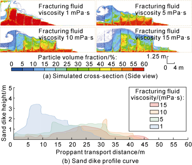
Fig. 11. Effect of fracturing fluid viscosity on the morphology of the main fracture sand dike. |
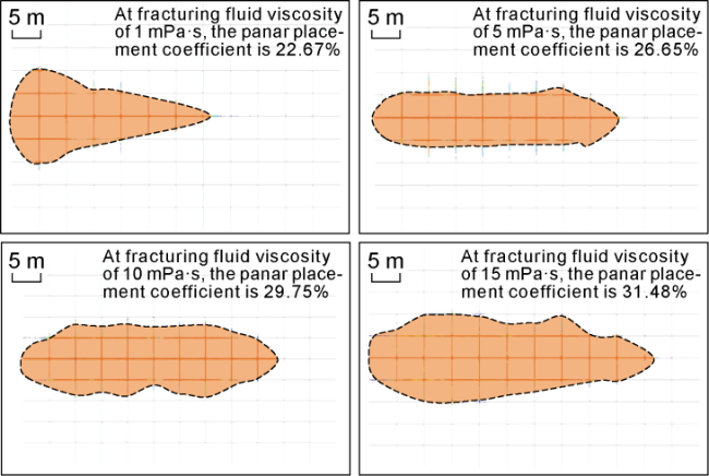
Fig. 12. Effect of fracturing fluid viscosity on planar placement efficiency (top view). |
3.3.4. Impact of pump rate
The pump rate was varied to 0.5, 1.0, 1.5, and 2.0 m3/min to simulate its impact on proppant placement efficiency. The simulation results are obtained as follows. At a low pump rate (e.g., 0.5 m3/min), the sand-carrying capacity of the fracturing fluid is limited, resulting in a relatively short proppant transport distance and primarily depositing near the wellbore, forming a relatively high sand dike. In this scenario, the effective support length of the sand dike within the main fracture is 28.50 m. As the pump rate gradually increases (e.g., 2.0 m3/min), the sand-carrying capacity of the fracturing fluid improves correspondingly, and the proppant transport distance continues to increase. Consequently, the effective support length of the sand dike within the main fracture reaches 48.14 m (Fig. 13). The higher the pump rate, the larger the proppant transport distance in the main fracture, the wider the placement range, and the higher the planar placement coefficient. When the pump rate is 0.5 m3/min, the planar placement coefficient is only 14.83%. When the pump rate reaches 2.0 m3/min, the planar placement coefficient increases to 29.01%, representing an improvement of 14.18 percentage points (Fig. 14). Nonetheless, when the pump rate reaches a certain level (e.g., 2.0 m3/min), although the proppant transport distance increases and the placement range expands, the peak height of the near- wellbore sand dike decreases significantly, and the support effect at the near-wellbore end deteriorates. Therefore, in engineering applications, it is advisable to appropriately control the pump rate to ensure good support effects, or to implement a strategy with high-rate injection in the early stage and a low-rate injection in the later stage, balancing transport distance and support effectiveness.
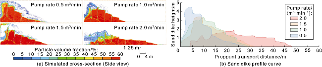
Fig. 13. Effect of pump rate on the morphology of the main fracture sand dike. |
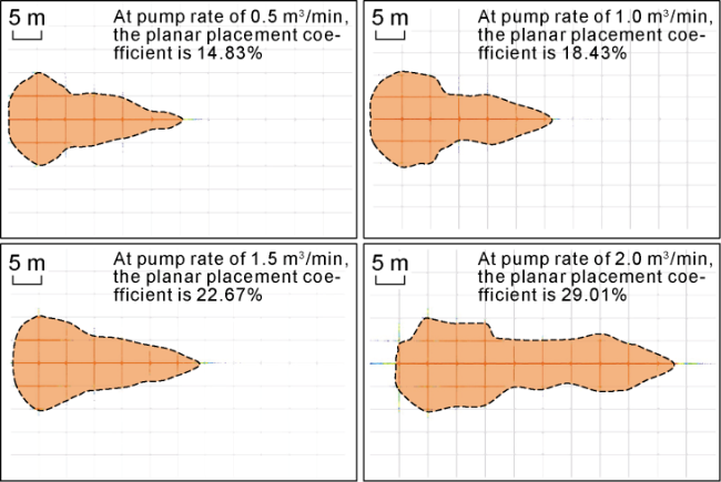
Fig. 14. Effect of pump rate on planar placement efficiency (top view). |
3.3.5. Impact of included angle between main and branch fractures
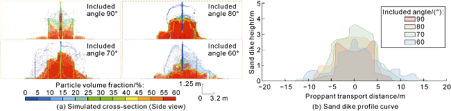
The included angle between the main and branch fractures was varied to 90°, 80°, 70°, and 60° to simulate its impact on proppant placement efficiency. The following findings are revealed. When the main and branch fractures are oriented vertically (at a 90° included angle), the fracturing fluid experiences a relatively low flow resistance in the main fracture due to its larger aperture compared with branch fractures. Under inertia, proppants tend to continue flowing along the main fracture, resulting in a poor diversion capability into the branch fractures. Consequently, proppants primarily accumulate in the main fracture, with the planar placement coefficient of only 22.67%. As the included angle decreases, the geometric connection between the main and branch fractures changes, enhancing the fluid’s ability to enter the branch fractures. This allows more fluid and proppant to flow into the branch fractures, effectively expanding the planar placement range. At an included angle of 60°, the planar placement coefficient reaches 31.04% (Fig. 15), an increase of 8.37 percentage points. The smaller the included angle between the main and branch fractures, the stronger the proppant’s transport ability within the branch fractures, leading to longer sand dikes. When the included angle is 90°, the effective length of the sand dike formed in the branch fracture is only 17.1 m. At an included angle of 60°, the effective length of the sand dike in the branch fracture reaches 28.2 m, an increase of 64.91% (Fig. 16). In summary, when the included angle between the main and branch fractures is small, proppants can form long, widespread and uniform sand dikes in the branch fractures, which is more conducive to effective support. Conversely, when the included angle is large, the proppant’s transport distance in the branch fracture is limited, leading to accumulation near the entrance of the branch fracture and a significant reduction in effective support range.
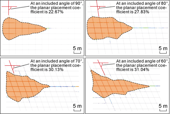
Fig. 15. Effect of included angle on planar placement efficiency (top view). |
Fig. 16. Effect of included angle on the morphology of the main fracture sand dike. |
4. Conclusions
The proppant transport in the fracture network can be divided into three stages: initial filling, dominant channel formation, and fracture network extension. In the initial filling stage, patchy accumulation primarily occurs in the near-well region. In the dominant channel formation stage, sand dike narrowing leads to the formation of multiple dominant channels, with proppants preferentially placed along the main fracture. In the fracture network extension stage, the flow velocity in the main fracture decreases, fluid diverts to secondary fractures, and the planar placement coefficient increases.
Higher proppant density, lower fracturing fluid viscosity, lower pump rate, and larger proppant particle size result in poorer suspension and carrying capabilities of the fracturing fluid for proppants, leading to shorter transport distances and lower planar placement coefficients for proppants, and vice versa. In engineering applications, to expand the stimulation range, it is recommended to use low-density, small-particle proppants in conjunction with high-viscosity fracturing fluids, while appropriately increasing the pump rate.
A smaller angle between the main and branch fractures results in longer sand dikes formed in the branch fractures, broader placement range, more uniform distribution, and better stimulation effects. Conversely, a larger angle increases the likelihood of proppant accumulation near the entrance of the branch fractures, resulting in a lower planar placement coefficient.
Nomenclature
a—acceleration of a particle per unit mass, m/s2;
Cs—smagorinsky constant, dimensionless;
dp—particle diameter, m;
Dp—particle drag coefficient, s-1;
Ff—buoyancy force on the particle phase, N;
g—gravitational acceleration, m/s2;
i, j—stress directions;
I—cell number along the x-axis;
k—grid cell index;
l—particle cluster number within a grid cell;
LF—filtering scale, m;
mp—mass of a single particle, kg;
n—time step;
np—total number of particles in each cluster;
Np—total number of particle clusters;
O—interpolation operator, dimensionless;
Ok—interpolation operator at cell k, dimensionless;
Ox, Oy, Oz—components of the interpolation operator in the x, y, z directions, dimensionless;
OI,x—component of the interpolation operator of cell I in the x direction, dimensionless;
p—fluid pressure, Pa;
ps—coefficient of particle stress dependence on particle volume, Pa;
Qp, Qk—variable placeholders, in units depending on the physical quantity they represent;
r—particle radius, m;
Re—particle Reynolds number, dimensionless;
Sij—strain rate component, s-1;
—filtered strain rate tensor, s-1;
t—time, s;
u—velocity vector, m/s;
ui, uj—velocity components in the i, j directions, m/s;
uf, up—fluid phase and particle phase velocities, m/s;
—average particle phase velocity, m/s;
uf,p—fluid velocity at the particle's location, m/s;
wp—spatial coordinates of a point in the particle phase, e.g., xp, yp, zp;
x, y, z—spatial coordinate system, m;
xi, xj—spatial coordinate components in the i, j directions, m;
αcp—maximum accumulation volume fraction of dense phase particles, %;
αf, αp—volume fractions of the fluid phase and particle phase, %;
αpk—volume fraction of the particle phase in cell k, %;
χ—empirical coefficient, %;
βfp—interphase momentum exchange rate per unit volume, N/m3;
βk—interphase momentum exchange rate at grid node k, N/m3;
vt—eddy viscosity coefficient, m2/s;
δij—Kronecker delta symbol, dimensionless;
λd—drag coefficient, dimensionless;
μf—fluid phase viscosity, Pa·s;
ρf, ρp—densities of the fluid phase and particle phase, kg/m3;
σp—normal stress of particles, Pa;
τij—stress component, Pa;
τf—stress tensor of the fluid phase, Pa;
τp—stress tensor of the particle phase, Pa;
—filtered subgrid-scale fluid stress tensor, Pa;
—particle distribution probability function, m-3;
—coefficient of the drag term, kg/(m3·s);
Ωp—particle volume, m3;
Ωk—volume of cell k, m3;
ε—small number (order of 1×10⁻⁷) used to eliminate singularities;
—Hamiltonian operator, spatial derivative, m-1;
—velocity space gradient operator, s/m;
“~”—spatial filtering operation function, and variables marked with this symbol above indicate the corresponding variable after filtering.