Nuclear magnetic resonance (NMR) logging data plays a very important role in obtaining reservoir parameters, pore structure and fluid types of complex and unconventional oil and gas reservoirs ^[1⇓-3]. Since relaxation signals are only related to the hydrogen atom in a porous medium, it is feasible to calculate the porosity, permeability, irreducible water saturation, pore radius, and the wettability index of the reservoir by measuring the signals of the macroscopic magnetization vector of the hydrogen atom decaying with time, and inverting them to T₂ spectrums, and considering proper petrophysical models. Then the quality and pore structure of the reservoir can be evaluated by the inverted T₂ spectrums ^[1⇓-3]. And finally, quantitative data such as the fluid types, fluid saturations and fluid viscosities will be obtained by using multidimensional data such as the longitudinal relaxation time, diffusion coefficient and internal magnetic gradient of the reservoir ^{[4⇓⇓⇓-8]}. Compared with conventional well logging data such as GR, AC, and compensated DEN, T₂ spectrums include richer geological information.

Limited by international technical support and field operating conditions, NMR logging data recorded in most oilfields in China are only one-dimensional T₂ data. It is vital to make a great use of conventional T₂ spectrums to solve the petroleum and geological problems. Many scholars conducted substantial investigations on the applications of NMR logging data and made great achievements on estimating porosity, permeability, irreducible water saturation, T₂ cutoff value, as well as T₂ calibration of pore size ^[9⇓⇓-12]. In addition, some innovative researches on interpretation of T₂ spectrums were proposed, including pore structure indication based on the concentration of T₂ spectrum distribution, quantitative T₂ spectrum analysis based on mathematical morphology, multifractal analysis of T₂ spectrums, key parameter extraction based on multi-Gaussian function fitting, as well as machine learning techniques such as self-organizing maps neural network, non-negative matrix factorization, and independent component analysis ^{[13⇓⇓⇓⇓⇓⇓⇓⇓⇓⇓-24]}.

These methods provide new ideas for the interpretation of NMR logging data. However, there are some obvious drawbacks. Firstly, it is still difficult to describe the nonlinear response between pore structure and NMR response. Secondly, data manipulation and parameter setting should be calibrated with experimental results or manually. To this end, we propose a novel method to process NMR logging data based on the Gaussian mixture model (GMM). It is an unsupervised technique that the clustering result is objective. Both numerical simulation and field NMR logging data have been used to demonstrate the method.

The GMM is the extension of univariate Gaussian distribution in high dimensional space. It is the linear combination of finite independent multivariate Gaussian distribution models. As a probability model with the fastest learning ability, it constructed an optimal mixed multidimensional Gaussian distribution model by fitting input dataset, so we can get unsupervised clustering results, consequently data distribution pattern, and classification scheme. The clustering method based on the GMM is widely used in many areas such as image segmentation, signal processing, biomedical science, and geosciences ^{[25⇓⇓⇓⇓⇓-31]}. According to the concept of the GMM^{[26⇓⇓-29]}, the probability distribution of a logging dataset can be expressed by Eq. (1) to Eq. (3).

The purpose of the GMM clustering is to solve the mean, variance, and weight for each Gaussian basis function, which is usually achieved by the expectation maximization (EM) algorithm. The basic idea of the EM algorithm is to maximize the likelihood function for problems with latent variables and some iteration equations ^{[26,31⇓ -33]}. It is often using the logarithmic form of the likelihood function (Eq. (4)), in order to simplify the computation. Therefore, the problem is then transformed to find the maximal value of the logarithmic form of the likelihood function, which is expressed by Eq. (5).

The EM algorithm can be separated into two steps. The first step obtains the expectation value (E step) and the second step obtains the maximum value (M step). The specific iterative procedures are as follows: (1) Initialize the model parameters, let the mean M_k as a random matrix, the variance matrix D_k as an identity matrix, and the weight matrix W_k as the prior probability for each model. (2) Obtain the prior probability belonging to each Gaussian model at each depth (or measured point), which can be expressed as Eq. (6). (3) Update the model parameters using the prior probability and Eq. (7) to Eq. (9). (4) Repeat Step 2 and Step 3 until satisfying the convergence criteria of Eq. (10).

Determination of the optimal number of the Gaussian models is imperative to this algorithm. If the number is too large, it is easy to cause the overfitting. However, if the number is too small, it is easy to reduce the flexibility of fitting new data. The frequently used method to over these drawbacks is to introduce the Akaike information criterion (AIC). Based on the information entropy, the AIC can help us to choose the models with the minimum information loss ^{[34⇓⇓-37]}, which is expressed in Eq. (11).

The AIC is the basis of determining the optimal number of the Gaussian models. Moreover, sometimes the AIC is monotonically decreased with the number of the Gaussian models. Therefore, it is practical to use the variation of the AIC for the optimal number, increasing the sensitivity between the AIC and the optimal number of the Gaussian models to some extent ^[38].

We adopt the variation of the AIC to quantify the optimal number of the Gaussian models, which is expressed in Eq. (12). If the variation of the AIC is too large when increasing the number of the Gaussian models from p to p+1, it is inferred that p is not enough to depict the original dataset. Otherwise, the clustering results are similar for p and p+1. We can choose p as the optimal number from the perspective of computation cost, and the corresponding variation of the AIC will reach its minimum value.

As is stated above, T₂ spectrums are the coupled responses of many petrophysical properties such as pore structure and fluid components. The T₂ spectrum measured at each depth follows Gaussian distribution and indicates the distribution of relaxation components. We can use the GMM algorithm to process T₂ spectrums and obtain unsupervised clustering results, which will be used for pore structure evaluation and reservoir classification.

Before the GMM clustering, it is necessary to compress the big NMR data by principal component analysis (PCA) to reduce the relevance between the data and enhance the computation efficiency. In doing so, firstly, we should evaluate the adaptability and effectiveness of the GMM clustering method through numerical simulation, and then generalize the method to process raw NMR logging data.

T₂ spectrums can be viewed as a matrix that is composed of the amplitudes of different relaxation times, and the column (or the dimension) of the matrix is dependent on the number of inversion points. The amplitudes corresponding to different relaxation times have certain correlations. To reduce the redundant information in the T₂ spectrums and highlight the analyzable factors, we used PCA algorithm to compress the high dimension data to low dimension and extract the most representative principal components ^[38-39].

Assuming the number of inversion points is L and the number of measured points is M, T₂ spectrums can be expressed as an observation matrix, seen in Eq. (13). Since the column vectors corresponding to different relaxation times have certain correlations, it is feasible to transform the observation matrix to a new matrix with a few linearly uncorrelated columns that contain the largest amount of information, and to improve the computation efficiency by PCA. The original observation matrix can be converted by Eq. (14) and Eq. (15).

The basic principle and the computation method of the PCA algorithm can be seen in references [38⇓-40]. The specific steps are as follows: (1) Normalize the raw data; (2) Calculate the correlation matrix to obtain the eigenvectors and the eigenvalues; (3) Compute the cumulative variance contribution rate according to the distribution of eigenvalues; (4) Set the cut-off value of contribution rate and extract the principal component signal.

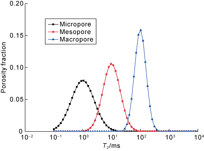
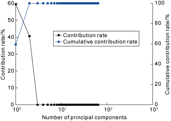
We used three log Gaussian functions to simulate 400 groups of T₂ spectrums (Fig. 1). The purpose of these log Gaussian functions is to control the peak value and the distribution range. In our forward model, the peak values are 1, 10, and 100 ms, the variances are 0.4, 0.3, and 0.2. Moreover, the relaxation time is defined from 0.1 ms to 10000 ms with 64 logarithmic uniform grids. The amplitudes of T₂ spectrums are generated randomly and then normalized to reduce the influence of the porosity. When pore fluid is water, the T₂ spectrums can represent micropores, mesopores and macropores. The statistical results show that the relaxation time of the micropore ranges from 0.1 ms to 14 ms, the relaxation time of the mesopore ranges from 1.3 ms to 86 ms, and the relaxation time of the macropore ranges from 24 ms to 372 ms. Fig. 2 shows the relationship between the number of principal components and the contribution rate, and the cumulative contribution rate. It is observed that the cumulative contribution rate can reach as high as 99.95% when the number of principal components is 2, indicating that there is a high correlation between the column vectors (or amplitudes) corresponding to different relaxation times. It only needs to choose the first two principal components for the GMM clustering algorithm.

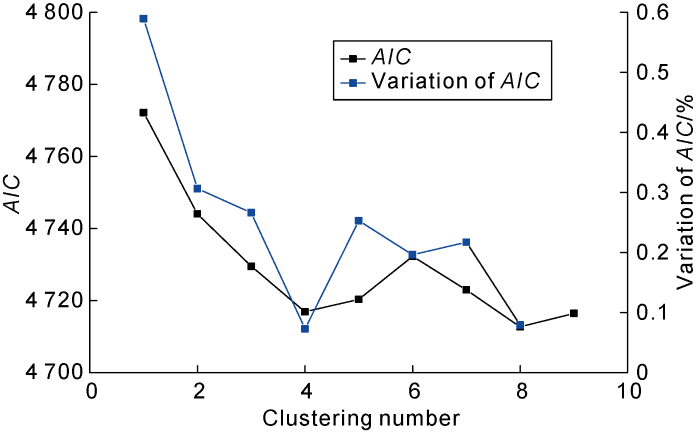
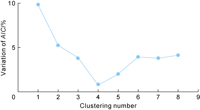
After dimension reduction by PCA, we used the first two principal components as the input data to conduct the GMM clustering driven by the EM algorithm. In the computation, the iteration threshold was 0.01, the maximum iteration number was 10 000, and the maximal clustering number (or the number of the Gaussian models) was 9. Fig. 3 shows the AIC and the variation of the AIC at different clustering numbers. It is seen that the variation of the AIC has reached its minimal value (0.073%) when the clustering number is 4, revealing the optimal fitting result has been fulfilled. Considering the fitting accuracy and computation cost, we chose 4 as the optimal clustering number.

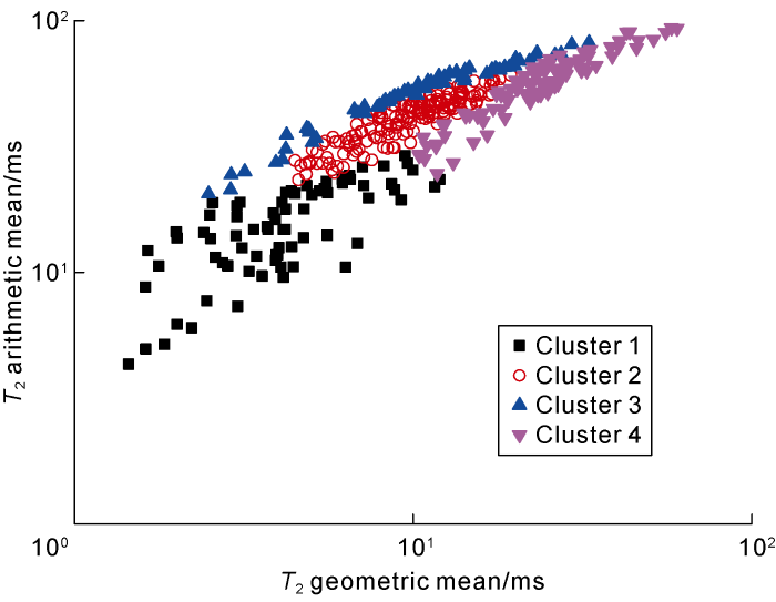
We computed the T₂ geometric mean and the T₂ arithmetic mean of these four clusters and obtained their crossplot, as shown in Fig. 4. It is obvious that both the T₂ geometric mean and the T₂ arithmetic mean are increased with from Cluster 1 to Cluster 4. However, they are less distinct from Cluster 2 to Cluster 4, indicating that it is difficult to classify the clusters simply using the conventional T₂ average value or conventional crossplot.

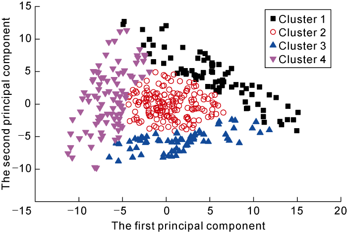
Fig. 5 shows the crossplot of the first and the second principal components for all clusters. Compared with Fig. 4, the distinction is more obvious, further verifying the reasonability of the clustering results based on the GMM clustering algorithm.

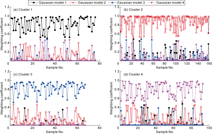
Fig. 6 displays the distribution of the weighting coefficients of the Gaussian models corresponding to four clusters. It is seen that the weighting coefficients correspond well with the clusters. Through the GMM clustering algorithm, we can get the clustering results, can assign the membership of the clusters precisely based on the probability distribution. The GMM clustering algorithm provides flexible cluster shape and the probability of the data belonging to different clusters. It can avoid hard classification effectively and bring more information than the hard-clustering algorithms ^[30].

Integrating the above algorithms, we processed the numerical simulated NMR logging data and obtained the following results (Fig. 7). Compared with conventional NMR logging interpretation profiles, our method can provide quantitative GMM clustering results and the probability distribution of different clusters, which give intuitive information.

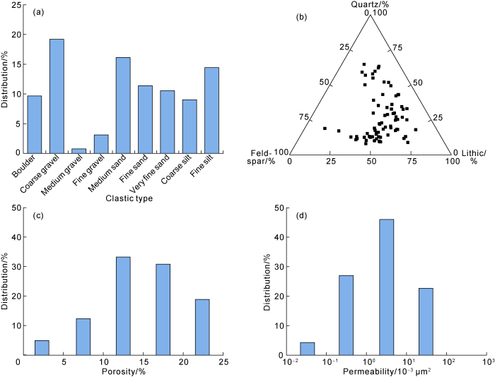
The Niudong area is located in the eastern front of Altun mountain in the northwest Qaidam Basin. The Jurassic formation in the Niudong area is typical braided delta plain sediment which is mainly composed of medium to coarse sandstones including feldspathic lithic sandstone or lithic arkose filled with kaolinite and calcite at a low content (Fig. 8). The reservoir space is mainly composed of secondary pores, followed by intergranular pores, which are uniformly distributed and well connected. The reservoir physical properties are relative good: the porosity is from 5% to 20%, and 11.3% on average; and the permeability is (0.1-100.0)×10^-3 μm², and 5×10^-3 μm² on average (Fig. 8).

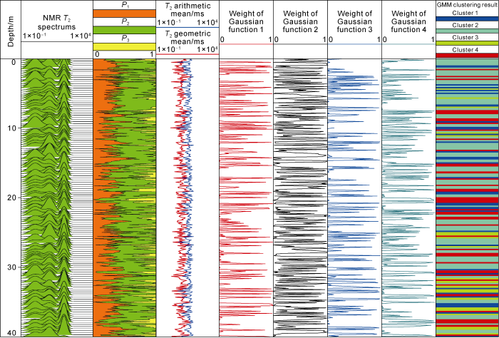
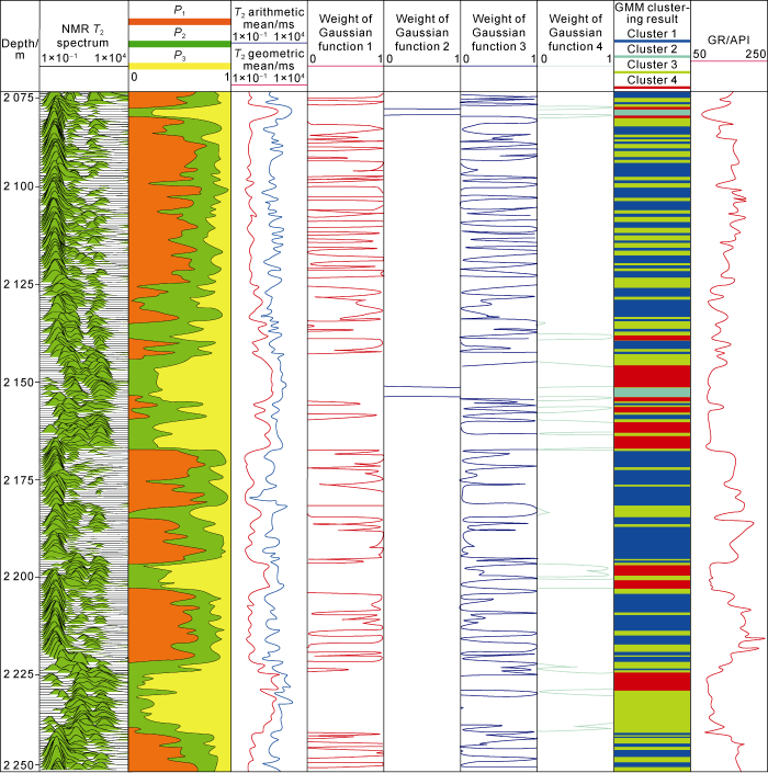
Using the D9TW model, NMR logging data were acquired in Well XX-1 well using a MRIL-P logging tool manufactured by Halliburton. We obtained the standard T₂ spectrums from the data acquired with long waiting time (12.988 s) and short echo spacing (0.9 ms). Setting the threshold of the cumulative contribution rate as 90%, we compressed the observation matrix of 64 columns to 7 principal components by PCA. Using the GMM clustering algorithm to these 7 principal components, we obtained the relationship between the variation of the AIC and the number of the Gaussian models (Fig. 9). Finally, we fixed the optimal cluster number to be 4 according to the criteria mentioned above. Applying 0.3, 10 and 100 ms as cut-off values, we obtained the proportions of the amplitude in the relaxation range of 0.3 to 10 ms (namely P₁), the relaxation range of 10 to 100 ms (namely P₂), and the relaxation range higher than 100 ms (namely P₃) (Fig. 10).

Fig. 11 shows the proportions of the amplitude for 4 relaxation ranges agree well with the clustering results. Cluster 1 has the maximal P₁ and the minimal P₃, indicating the development of micropores. Cluster 2 has the maximal P₃ and the minimal P₁, indicating the development of macropores. Clustering 3 has the complicated distribution of the relaxation components. Cluster 4 has similar distribution as Cluster 2.

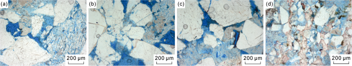
Three intervals were tested in the Jurassic formation drilled in Well XX-1. From the section from 2074.5 m to 2082.5 m, open-flow gas production at 2422 m³/d was obtained through a 6-mm nozzle after fracturing stimulation. It is a low-yield gas layer belonging to Cluster 3 according to the GMM clustering algorithm. From the section from 2146.5 m to 2153.5 m, open-flow gas production at 132 942 m³/d and open-flow oil production at 13.27 t/d were obtained through a 10-mm nozzle. It’s a high-yield gas layer belonging to Cluster 4. From the section from 2228.5 m to 2240.5 m, open-flow gas production at 22 484 m³/d and open-flow oil production at 0.42 t/d were obtained through a 5-mm nozzle. It is a high-yield gas layer belonging to Cluster 4. Observed on typical thin sections from drilled cores in the section from 2228.5 m to 2240.5 m (Fig. 12), the grain size is relatively large and the lithology is mainly particle-supported (gravelly) giant to coarse-grained feldspathic lithic sandstone. The particles are subangular and contact each other point to point. The cementation type is mostly pore cementation. The quartz surface is clean and observed wavy extinction. The feldspar is strongly weathered. The pores are mainly intergranular dissolved pores, intragranular dissolved pores and matrix micropores. In addition, the shale interval from 2096 m to 2103 m (showing high GR readings) belongs to Cluster 1.

We proposed a quantitative method to get unsupervised clustering results of NMR logging T₂ spectrums using the GMM clustering algorithm. To improve the computational efficiency, we compressed the NMR T₂ data using the PCA method before clustering. Moreover, we adopted the AIC criteria and the variation of the AIC to determine the optimal number of the Gaussian models and the clusters, which can enhance the validity of the clustering results. The method we proposed has been verified by both numerical simulation and field NMR logging data. The result shows that the clustering results agree well with the pore structure, reservoir type and production capacity of the reservoir analyzed. And the quantitative characterization results can directly reflect the reservoir type and pore structure.

It should be noted that the influences of fluid properties were not considered in our numerical simulation. Real NMR response and its T₂ spectrum are affected by various factors such as lithology, fluid and pore structure, which should be considered in future studies. Moreover, if the GMM clustering algorithm is used after typing lithology or constrained by other information such as petrophysical, well test and production data, the clustering result and its reasonability may be improved to some extent.

AIC—Akaike information criterion;

d—physical dimension of well logging data;

D_k—variance matrix of the k-th Gaussian basis function;

i—sequence number of well logging data;

j—number of iteration;

k—sequence number of Gaussian basis functions;

L—point number on T₂ spectrum of NMR logging;

M—sample number of well logging data;

M_k—mean matrix of the k-th Gaussian basis function;

N—total number of Gaussian basis functions;

p—cluster number;

p(X)—total probability density function;

W_k—weight matrix of the k-th Gaussian basis function;

X—matrix of well logging data;

Y—component matrix corresponding to logging data;

U—basis matrix corresponding to logging data;

θ(X)—logarithmic likelihood function;

θ(X)_j—logarithmic likelihood function after the j-th iteration;

φ(X, M_k, D_k)—probability density function of the k-th Gaussian basis function;

ε—iteration threshold of logarithmic likelihood function;

Θ(X)—the maximum of logarithmic likelihood function.