Underbalanced drilling (UBD) is a kind of high-efficient drilling method. In UBD, gas is injected into the drilling mud to regulate bottom-hole pressure (BHP). When solid particles (cuttings) are added, the gas-liquid mud two-phase flow in the annular space of the wellbore turns into the gas-liquid-solid three-phase flow. In drilling operation especially in deep formations, the drilling fluid inside the wellbore changes in temperature due to heat transfer between the drilling fluid and surrounding formation. Since the drilling fluid properties are closely related to the temperature, accurate calculation of the fluid temperature profile is related to the accurate prediction of the pressure profile and BHP.

Many researchers have studied heat transfer in wellbore and used numerical and analytical methods to calculate the drilling fluid temperature. Ramey ^[1], Holmes and Swift ^[2], Arnord ^[3], and Kabir et al. ^[4] solved the energy equations by half transient method which assumed that heat transfer inside the formation was transient and that inside the wellbore was steady. Raymond ^[5] established numerical models for the first time to predict fluid temperature profile during both transient and pseudo-steady-state conditions. Marshall and Lie proposed a numerical model of single-phase flow to calculate the steady-state and transient temperature profiles in the wellbore by using a finite difference approach ^[6]. Song et al.^[7] obtained the pressure and temperature profiles of circulating gas-liquid two-phase flow in well by using a homogeneous model which took the effects of viscous dissipation, drill-string rotation and drill bit energy into account. Perez-Tellez et al. ^[8-9] proposed a mechanistic model to assess BHP and pressure profile in the wellbore during drilling. Khezrian et al. simulated gas-liquid

two-phase flow in the annulus during UBD with a steady two-phase flow model considering the effect of geothermal temperature gradient ^[10]. Shekari et al. simulated two-phase flow in the annulus of the wellbore during UBD with a transient two-phase flow model ^[11]. Ghobadpouri et al. solved governing equations of two-phase (gas-liquid) flow in the annulus during drilling which considered geothermal temperature gradient and fluid production from the reservoir into the annulus, but didn’t consider the effects of cuttings and heat transfer between the drilling fluid and the surrounding formation on the pressure distribution and BHP ^[12]. Ghobadpouri et al. simulated gas-liquid-solid three-phase flow in the annulus using a 1D steady-state three-phase flow model, and proved that the three-phase model gave more accurate BHP results than the two-phase model ^[13]. But the effects of heat transfer between the drilling fluid and the surrounding formation on pressure distribution and the BHP were not discussed in this study. Hajidavalloo et al. found that compared with two-phase flow with assumed geothermal temperature gradient, the two-phase flow model considering energy equation could predict BHP more accurately during UBD^[14]. Falavand-Jozaei et al. investigated key factors affecting temperature and pressure distribution of gas-liquid two- phase flow during under-balanced drilling operation^[15]. Hajidavalloo et al. examined the effect of temperature variation on the predicted bottom-hole pressure during drilling under single-phase flow condition ^[16].

As mentioned above, few numerical models considered the effect of temperature and the models are simple. Most of the numerical models did not consider the presence of solid phase in the annulus and the effect of solid phase on the heat transfer between liquid and formation, which are not the actual situation. The presence of cuttings and its heat transfer in the well may affect the BHP and impose restrictions on the controlling parameters of hole-cleaning. The effect of transient thermal interaction between drilling fluid containing solid particles and the formation has been considered in the three-phase flow model established in this work in order to get more accurate BHP predictions.

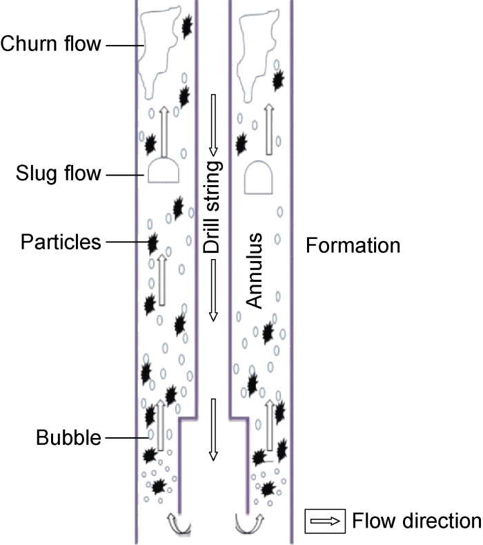
As shown in Fig. 1, in UBD operation, gas-liquid two phase flow is pumped down through the drill string, passing through the drill bit and carrying cuttings. The gas-liquid two phase flow, formation fluid and cuttings mix in the annulus into three-phase gas-liquid-solid flow and move upward. As the produced gas is very similar with the injected gas in thermophysical properties, it can be assumed that the formation gas and injected gas can be considered as a mixture which moves at the same velocity. Also, the injected liquid and formation liquid are assumed as a mixture which flows at the same velocity in the annulus.

The three-fluid model considers the individual velocity of each phase and was used to simulate gas-liquid-solid three-phase flow in the annulus. In this model, the liquid phase is assumed incompressible, the gas phase is assumed compressible, and the fluid in the wellbore is assumed one-dimensional. The turbulent shear stress and viscous effects are considered in the friction coefficients between the phases and between the phases and the wall. In this study, a steady one-dimensional gas-liquid-solid three-phase flow incorporating variable fluid properties is considered at each time-step in the drill string and annulus, whereas heat transfer between the wellbore and surrounding formation is considered transient since the temperature at any point will change with time during fluid circulation.

According to the above-mentioned assumptions, the continuity equation for each phase is as follows ^[17]:

The conservation of momentum equation for each phase is as follows ^[17]:

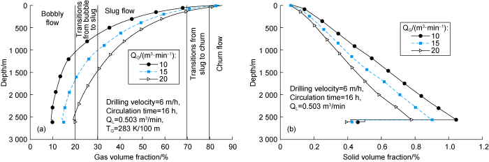
Flow pattern is determined based on the gas volume fraction value method proposed by Hatta et al. ^[18]. According to this method, flow pattern is bubbly if gas volume fraction is less than 20%; bubbly flow transitions to slug at the gas volume fractions from 20% to 30%, slug flow pattern is dominant when the gas volume fraction is between 30.00% and 69.15%; slug flow transitions to churn flow at the gas volume fraction between 69.15% and 79.15%; and finally at the gas volume fraction of greater than 79.15%, the churn flow is dominant. Ishii and Mishima relations are used to calculate F_ig and F_il forces according to the flow pattern ^[19]. Also, relations proposed by Drew et al.^[20] are used to calculate F_wg, F_wl, F_vg, and F_vl. Stuhmiller relation ^[21] is used to calculate the pressure correction term:

In addition, the solid particles mass flow rate can be calculated using drilling velocity as follows ^[22]:

Besides the conservation equations (Eqs. 1 and, 2), two additional equations are required to solve the pressure distribution. One is the gas equation of state and the other is the algebraic constraint. The algebraic constraint can be expressed as follows:

The gas equation of state is as follows:

Where Z is the gas compressibility factor, for which different relations can be used, in this paper, the Dranchuk and Abou-Kassem relations ^[23] are used.

As shown in Fig. 1, three different regions in the wellbore, drill string, annulus, and formation, have heat transfer. Energy conservation equation for a control volume inside the drill string can be obtained by adding the source term to the Osisanya and Harris energy equation as follows^[24]:

The first term on the left-hand side of Eq. 7 represents the heat transfer between the fluid inside the drill string and fluid in the annulus, the second term represents the net rate of energy transfer to the control volume by the bulk flow of fluid, the third term represents the source term inside the drill string, and the right-hand side of Eq. 7 represents the accumulation of energy within the control volume inside the drill string.

Energy conservation equation for a control volume inside the annulus can be obtained by adding the source term to the Osisanya and Harris energy equation^[24] as follows:

Similarly, the terms on the left-hand side of Eq. 8 are the heat transfer from the formation to the annulus fluid through convection, the heat transfer between the fluid inside the annulus and that in the drill string, the net rate of energy transfer to the control volume by the bulk flow of fluid, and the source term inside the annulus, respectively. Also the right-hand side of Eq. 8 represents the accumulation of energy within the control volume inside the annulus.

U_p is the overall heat transfer coefficient between fluid inside the drill string and the fluid in the annulus, and its calculation formula is as follows:

In Eq. 9 the convection heat transfer coefficients can be calculated from Rezkallah and Sims relation, the accuracy of this relation is improved by using the relation proposed by Kim ^[25]:

In the Eq.10, the exponent “n” has different values according to the flow pattern: n=-0.76 for the bubbly flow, n=-0.62 for the slug flow, n=-0.43 for the churn flow, and n=-0.65 for the annular flow. h_lsp is liquid single-phase heat transfer correlation coefficient proposed by Kim, see Reference [25] for its calculation method in detail:

S_p and S_a in Eqs. 7 and 8 are the source term inside the drill string and the annulus, which are given by Li et al., see Reference [26] for their relations:

Boundary conditions are as follows:

(1) For the surface: The inlet temperature into the drill string is given.

(2) For the well bottom: There are three types of boundary conditions to use as given by Al-Saedi et al.^[27]. In this study, the first kind boundary condition, or Dirichlet condition adopted by Gao et al. ^[28] is used, as at the bottom-hole, fluid temperature in the drill string and the annulus are equal.

Assuming a cylindrical geometry surrounds the wellbore, heat transfer to the formation can be described by an axis symmetric one- dimensional model. Based on this assumption, the diffusivity equation in the formation is expressed as follows:

The initial condition is:

The boundary conditions at the interface between the annulus and formation can be expressed as follows:

The left-hand side of Eq. 13 represents heat transfer between the formation and the annulus fluid through convection, and the right-hand side of Eq. 13 represents the heat conduction at the formation.

The boundary condition far from the wall can be expressed as follows:

First of all, under the steady-state flow condition, the temperature profile along the well can be estimated according to the geothermal temperature gradient, then the continuity and momentum equations are reduced to six ordinary differential equations. These six equations and Eq. 5 and Eq. 6 create a set of eight equations which has eight unknowns (3 velocities, 3 volume fractions, 1 pressure and 1 density of gas). Discretization of these equations results in a set of coupled nonlinear algebraic equations. These equations can be solved using Newton approach. See Reference [22] for the discretized forms of the equations.

The boundary conditions are: wellhead pressure is equal to the choke pressure, and the density of the gas at the wellhead is obtained from the gas equation of state. The velocities, pressure, and volume fractions can be calculated from the algorithm proposed by Bratland ^[22] using the Newton method.

The following is a summary of the steps taken in the numerical solution:

(1) The initial conditions of the system (t=0) are specified. The initial temperature conditions in the wellbore and formation are set according to the geothermal gradient. Then based on the temperatures of the fluids inside the drill string and annulus, the volume fractions, velocities, and pressure are calculated using the above set of equations.

(2) The temperature profile inside the drill string is estimated using Eq. 7 and the boundary condition at bottom-hole. It is necessary to assume the temperature of annulus fluid at the current time step in order to estimate the temperature profile inside the drill string. The temperature profile of annulus fluid at the previous time step is taken as the initial assumption.

(3) Based on the newly estimated temperature of the fluid inside the drill string, the temperature profile of annulus fluid is estimated using Eq. 8 and the boundary condition at bottom-hole. Similarly, it is necessary to assume the temperature profile in the adjacent formation at the current time-step. The temperature profile in the previous time step is taken as the assumed temperature profile.

(4) The formation temperature is then calculated using Eq. 11 at the current time step based on the newly estimated temperature profile of the annulus fluid. The results of this procedure are then compared with the initial assumption. If the error is acceptable, the next time step is run. Otherwise, based on the newly estimated temperature profiles of the fluids inside the drill string and annulus from steps 2 and 3, the volume fractions, velocities, and pressure are calculated again using the set of equations. And then the whole procedure is repeated using current temperature profiles in the annulus and formation as the new assumptions. This procedure is repeated until the calculations are completed for the total circulation time.

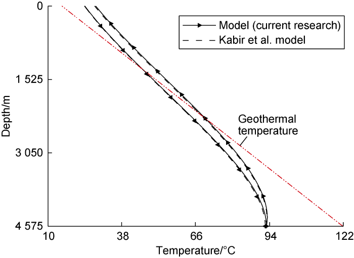
The model proposed in this paper was validated by comparing with Kabir et al. models ^[4]. Fig. 2 shows the temperature profiles of the fluids inside the drill string and annulus versus well depth after 44 hours of fluid circulation. The temperature profile obtained by the model proposed in this paper is in good agreement with the results from the Kabir et al. models, with a maximum error of about 0.3%.

Pressures and temperature predicted by using the three-phase flow model proposed in this paper have been compared with the field data of Well Muspac 53.

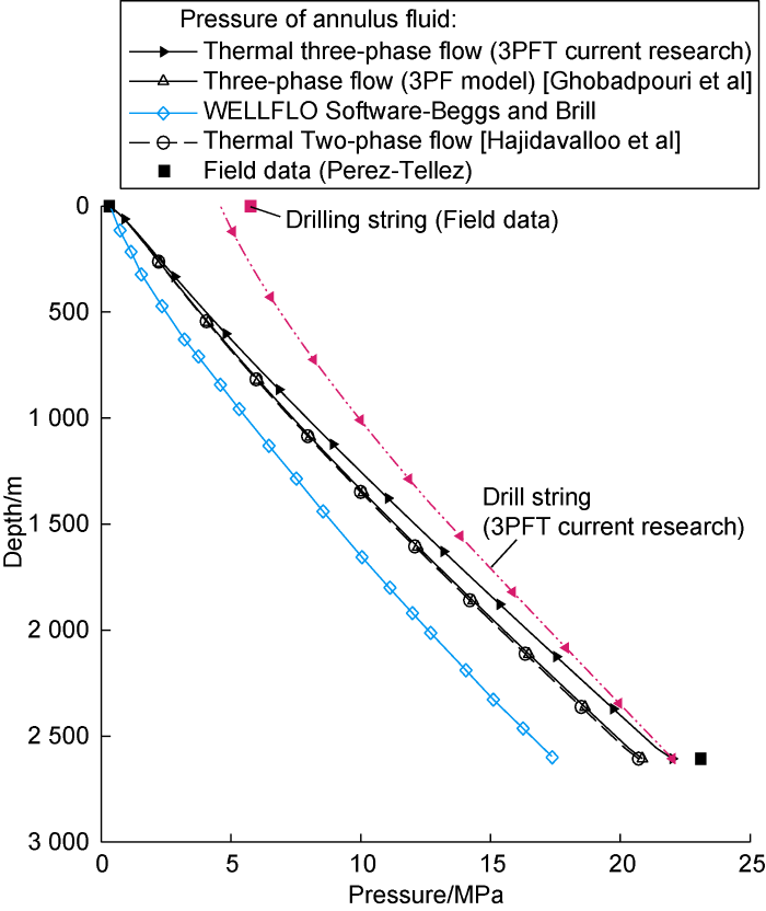
Fig. 3 shows the pressure distribution curves versus depth simulated by using different models. The basic calculation conditions in these simulations are: geothermal gradient of 0.028 3 K/m, drilling velocity of 6 m/h, and fluid circulation time of 16 hours. Fig. 3 clearly shows that the 3PFT model presented in this paper gives more accurate results compared with the three-phase flow model proposed by Ghobadpouri et al.^[13], two-phase flow model considering thermal conduction proposed by Hajidavalloo et al. ^[14], and other two-phase flow models including the WELLFLO software ^[29]. Predicted BHP by using 3PFT and 3PF models were compared with the field data, which shows that the BHP predicted by the 3PFT model has an error of 5.7%, while the BHP predicted by the 3PF model has an error of 11.3%, proving the accuracy of the model presented in this paper.

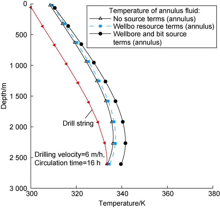
Fig. 4 shows the effects of source terms (internal heat generation) including viscous dissipation in the wellbore, friction between the rotating drill string and the wellbore wall, and heat generation by the drill bit in the calculations after 16 hours of fluid circulation. This figure confirms the necessity of including internal heat generation in the conservation of energy equation, as ignoring the effect of source terms results in predicted bottom-hole temperature (BHT) 6.1 K lower than then the actual BHT.

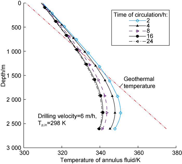
Fig. 5 shows the annulus fluid temperature profiles at different circulation moments and constant drilling velocity of 6 m/h. The annulus fluid temperature in the lower part of the wellbore changes significantly as circulation time increases. Moreover, the change of temperature is very rapid initially, and slows down later. As shown in Fig. 5, the formation temperature is much higher than the temperature of annulus fluid at the bottom-hole, but they have little difference at the wellhead. Also, Fig. 5 shows that annulus fluid temperature does not reach its maximum value at the lowest point of the well. Since the annulus fluid temperature is lower than the surrounding formation temperature, it receives heat from the surrounding formation. As far as heat gain of the annulus fluid is greater than heat loss to the fluid inside the drill string, annulus fluid temperature increases as it flows upward. However, as annulus fluid move upward, the rate of heat gain reduces as the annulus fluid encounters cooler formation temperature, while it still transfer heat to the cooler fluid inside the drill string. When the net heat gain equals the heat loss, the annulus fluid reaches its maximum temperature. In the studied case, the maximum temperature of annulus fluid after 16 h of fluid circulation, occurs at the vertical depth of 2251 m.

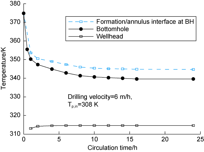
Variations of annulus temperature at the wellhead, bottom-hole, and bottom-hole temperature at formation/annulus interface versus circulating time are shown in Fig. 6. It can be seen in this figure that the temperature at formation/annulus interface and temperature of annulus fluid at the bottom hole decrease rapidly with the increase of time; but their drops begin to slow down when their difference is about 4 K later; they do not vary with circulation time after about 16 h of circulation. In the initial stage, the temperature of annulus fluid at wellhead increases with time, and then it reaches a constant value after approximately 4 h.

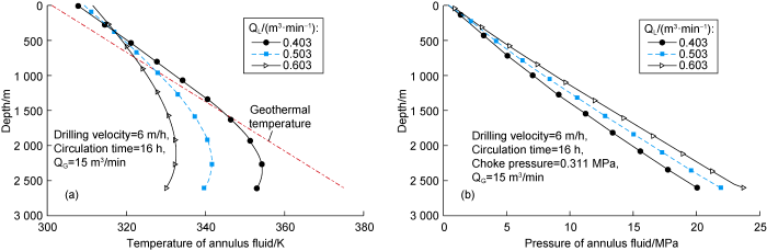
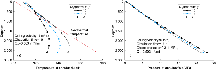
Figs. 7 and 8 show the effect of flow rates of liquid and gas on annulus fluid temperature and pressure profiles. Fig. 7a that the annulus fluid close to the wellhead increases in temperature but annulus fluid close to the well bottom decreases in temperature with the increase of the liquid flow rate. Since increasing the liquid flow rate makes the specific heat of the mixture increase, the temperature difference between the annulus fluid at bottom-hole and wellhead decreases. Fig. 7b shows that the BHP increases by about 1.76 MPa when flow rate of liquid increases from 0.503 m³/min to 0.603 m³/min. This is mostly due to increase in density of the mixture in the annulus. Fig. 8a shows that the annulus fluid close to the bottom-hole increases in temperature while annulus fluid close to the wellhead decreases in temperature with the increase of gas flow rate. Because gas has smaller specific heat than liquid, the mixture in annulus decreases in specific heat with the increase of gas flow rate, and the temperature difference between the annulus fluid at bottom-hole and wellhead increases with the increase of gas flow rate. Fig. 8b shows that the BHP decreases by about 0.76 MPa when the flow rate of gas increases from 15 m³/min to 20 m³/min. This is mostly due to density decrease of the mixture in the annulus with the increase of gas flow rate.

Fig. 9 shows the effects of gas flow rate on the distribution of gas and solid volume fractions with well depth. The gas volume fraction increases and the solid volume fraction decreases with reduction of well depth and also with the increase of gas flow rate. The sudden change in solid volume fraction at well bottom is due to the change of wellbore diameter. Therefore, the most critical part for hole-cleaning is the bottom of the well. Fig. 9a shows that flow pattern in the upper part of wellbore changes by increasing volume flow rate of gas.

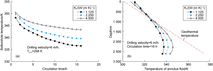
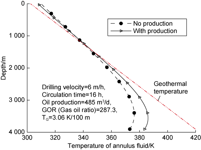
Fig. 10 shows the effect of thermal conductivity of the formation on temperature of annulus fluid at the well bottom over time. Fig. 10a shows that temperature of annulus fluid at the bottom-hole increases significantly with the increase of formation thermal conductivity. Fig. 10b shows that the thermal conductivity of formation has more significant effect on the temperature of annulus fluid at the well bottom. Fig. 11 shows the effect of influx of reservoir fluid on the temperature profile of annulus fluid in Well Iride 1166 documented in Reference [8]. The temperature of annulus fluid at bottom-hole increases by about 10 °C when the reservoir fluid flows into the well. It should be noted that in this paper, except Fig. 11 that uses the data of Well Iride 1166 in Reference [8], all the other figures use data of Well Muspace 53 in Reference [8].

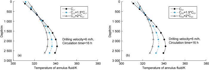
Fig. 12 shows the effects of specific heats of liquid and gas on the temperature profile of annulus fluid. Specific heat of the mixture increases with the increase of specific heats of liquid and gas. The figure shows that annulus fluid at the bottom-hole decreases in temperature while the annulus fluid at wellhead increases in temperature with the increase of specific heat of the mixture. It should be noted that the increase of gas specific heat has more significant effect on the mixture specific heat than the increase of liquid specific heat, this is because the specific heat of gas is smaller than that of liquid. Therefore, the higher the specific heat of gas, the lower the bottom-hole temperature, and the lower the risk of downhole tools failure will be. BHP increases by about 0.12 MPa and 0.17 MPa respectively when the specific heats of liquid and gas double.

Compared with other three-phase models only considering geothermal gradient (3PF) and two-phase flow models, The three-phase (3PFT) model considering heat transfer presented in this paper can predict BHP during UBD more accurately.

The heat produced by viscous dissipation, friction between rotating drill-string and well wall, and drill bit drilling, and influx of reservoir oil and gas have major effects on the temperature profile of the annulus fluid and consequently important effects on the BHP.

The fluid at the bottom-hole decreases in temperature with the increase of liquid flow rate, circulation time, and specific heats of liquid and gas, and increases in temperature with the increase of gas flow rate. BHP has stronger correlation with flow rates of liquid and gas, and the BHP increases with the increase of liquid flow rate but decreases with the increase of gas flow rate. BHP has weaker correlation with circulation time and specific heats of liquid and gas.

A—area, m²;

C—specific heat, J/(kg•K);

d—diameter, m;

F_g—gravity of unit volume, N/m³;

F_ij—interactive force between unit volumes, N/m³;

F_v—virtual mass force of unit volume, N/m³;

F_w—well wall friction of unit volume, N/m³;

G—geothermal gradient, K/m;

h—convection heat transfer coefficient, W/(m²•K);

h_lsp—heat transfer coefficient of liquid phase, W/(m²•K);

h_tp—convection heat transfer coefficient between two phases of the fluid, W/(m²•K);

k—thermal conductivity, W/(m•K);

M_g—molar mass of gas, kg/mol;

n—flow pattern index;

p—pressure, Pa;

Δp_ij—pressue correct term, namely, the pressure difference between pressure at phase interface and pressure inside the phase, Δp_is=0, Pa;

q—flow rate in mass, kg/s;

r—radius, m;

r_pi, r_po—inner and outer radii of drill string, m;

R—ideal gas constant, 8.314 J/(mol•K);

S—source term, W/m;

t—time, s;

T—temperature, K;

T_f—temperature at the interface of the formation and annulus, K;

U_a—overall heat transfer coefficient between the annulus fluid and formation, W/(m²•K);

U_p—overall heat transfer coefficient between fluid in drill string and fluid in annulus, W/(m²•K);

v—velocity, m/s;

v_d—drilling rate, m/s;

x—depth, m;

Z—gas compressibility factor;

α—volume fraction, %;

μ—viscosity, Pa•s;

ρ—density, kg/m³.

a—annulus fluid;

f—formation;

g—gas;

l—liquid;

p—fluid in drill string;

s—solid.