Introduction
Real-time identification of approaching bed boundary, one of the key techniques in logging-while-drilling (LWD) geosteering, is of great importance for accurate drilling and maximizing oil/gas production[1,2]. Although the formation boundary position can be predicted qualitatively from the responses of LWD Azimuthal Electromagnetic Measurements (AEM), these tool responses are usually very complicated due to the effects of complex downhole environments[3]. As a result, inversions of the AEM data are mandatory to quantitative evaluation of the distance between borehole and bed boundaries.
Generally, processing of electrical logging data acquired from high angle and horizontal well (HA/HZ) is a complex three dimensional (3D) inverse problem, in which multiple parameters, such as relative dipping angle, formation anisot-
ropy and invasion depth of mud filtrate, have to be considered[4,5,6]. If assuming the borehole and mud invasion are negligible and the formation property keeps invariant along one direction, the 3D data processing problem can be simplified into a two dimensional (2D) one[7,8]. To date, the 3D and 2D inversions are still impractical, since: (1) The amount and kind of measured electrical logging data are limited, which may result in some uncertainty in the inversed 3D and 2D outcomes; (2) There lacks of a fast 3D or 2.5D forward modeling algorithm; (3) The inversion involves too many parameters, so the computation load of Jacobian matrix is huge. To process the LWD electromagnetic (EM) data, the dimensionality reduction scheme with a sliding window technique is widely adopted in the industry. Yang et al. eliminated the abnormal apparent resistivity “horns” by ignoring the effect of lateral heterogeneity of the formation and using a simplified three-layered inversion model[9]. With the same inversion method, Li and Zhou extracted the nearby bed boundaries in real time[10]. Therefore, the complexity of inversion algorithm and inversion model can be reduced largely by simplifying the 3D inversion to a 1D question.
Selection of proper simplified inversion model and corresponding inversion method is critical to one dimensional (1D) processing of AEM data. Until now, the processing of AEM data is still limited to the dual-boundary model, whereas the suitability of dual-boundary model and feasibility of multiple-boundary model remain to be investigated. Generally, the choice of inversion algorithm is highly dependent on the complexity of the inversion model. The gradient methods have been extensively used for real-time processing of AEM data due to their limited iterations and fast inversion speed etc. However, the accuracy of gradient methods is highly dependent on the initial model. If an unsatisfactory initial model is used, incorrect inversion results may be obtained. Consequently, inappropriate geosteering decision may be made[11]. Compared with the dual-boundary model, multiple-boundary inversion involves more local minima of the cost function, and lacks of enough prior information, therefore gradient method is no longer suitable for this kind of inversion. By contrast, the stochastic Bayesian inversion method has been increasingly applied to the inversion of electrical data due to its global search capability and derivative free property[12]. To date, there is no report on Bayesian inversion used in the processing of AEM data. In addition, the convergence and speed of Bayesian inversion remain to be investigated.
This paper is organized as follows. First, high dimensional inversion problem of complex formation structure is simplified using the dimensionality reduction scheme, followed by the review of regularized Gauss-Newton algorithm and Bayesian optimization method. Then, for the simplified 1D inverse problem, the feasibility of various inversion models, the suitability of different optimization methods and the accuracy of inverted results are discussed. Best combination between the inversion model and inversion algorithm is also obtained. Finally, field example is presented to showcase the applications of the proposed inversion combination.
1. Theory of AEM and the dimensionality reduction scheme
1.1. Theory of AEM
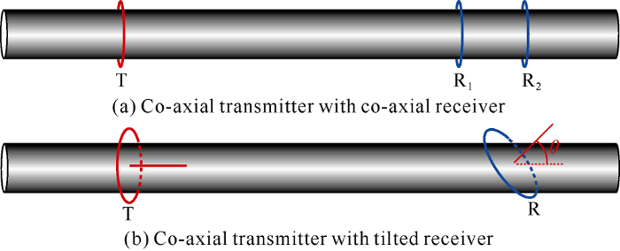
Taking the commercial tool PeriScope tool for example, the theory of AEM is reviewed in this section. PeriScope delivers two types of measures, i.e. apparent resistivities and geo-signals. As shown in Fig. 1(a), the former is constructed by measuring the voltages ${{V}_{{{\text{R}}_{1}}}}$ and ${{V}_{{{\text{R}}_{2}}}}$at two coaxial receivers R1 and R2 irradiated by a coaxial transmitter. The attenuation (Att) and phase shift (PS) are then extracted from the two voltages using Eq.1. Finally, the apparent attenuation resistivity and apparent phase shift resistivity are readily obtained by searching the resistivity values corresponding to the measured Att and PS from the pre-calculated convert chart.
Fig. 1.
Coil configuration of PeriScope.
The latter is acquired by a tilted coil which has a 45° with the tool axis. As the mandrel rotates, the voltages at different azimuthal angles are measured and the attenuation geosignal and phase shift geosignal are calculated using Eq.2.
1.2. Dimensionality reduction and inversion model
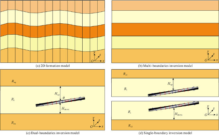
From the perspective of detection range of electrical logging measurement, the formation property can be assumed to be invariant along one direction, and therefore inversion of EM logging data of complex geological structures (e.g. folds) can be reduced to 2D, as shown in Fig. 2(a). For instance, the formation properties are inhomogeneous along x and y directions, while they are invariant along z direction. The 2D inversion problem can be further simplified to a combination of 1D ones by using the sliding window technique. As a result, the inversion speed has been improved significantly, since (1) In each sliding window, the analytical solution is used for the real-time forward modeling of the 1D formation model[13], and only 10-4 to 10-3 second is required for each logging point. (2) There are few parameters of interests in the simplified 1D inversion model. (3) The memory cost of 1D inversion can be ignored. For the inversion of ARM data, the 1D inversion models include multi-boundary model (Fig. 2b, with total layer number of more than 3), dual-boundary model (Fig. 2c, with total layer number of 3) and single-boundary model (See Fig. 2d, with total layer number of 2).
Fig. 2.
Dimensionality reduction of inversion model.
2. Gradient inversion and stochastic inversion
In this section, the commonly used gradient method, Gauss-Newton algorithm, is discussed, and the self-adaptive
multiplicative regularization term is also introduced to the cost function. Then, stochastic Bayesian algorithm is adopted to obtain the global optimum solution of complex model.
2.1. Multiplicative regularized Gauss-Newton algorithm
For the nonlinear inversion of ARM, the gradient method is used first. At kth iteration, the cost function ${{C}_{k}}\left( m \right)$ can be expressed as[14]
where, m is the model vector of inverted parameters and $F\left( m \right)$ is L2 norm between observed data ${{d}^{\text{obs}}}$ and simulated responses $S\left( m \right)$ given a formation model m,$F\left( m \right)=\frac{1}{2}{{\left[ S\left( m \right)-{{d}^{\text{obs}}} \right]}^{2}}$. ${{R}_{k}}\left( m \right)$is the self-adaptive regu-larization term given as:
where δ is a constant obtained from numerical experiments. ${{m}_{p}}$is the reference model vector which is usually set to the value of m at previous iteration,${{m}_{p}}={{m}_{k-1}}$.
The Gauss-Newton method is used to solve Eq. 3. At the kth iteration, setting the derivative of cost function to m equal to zero, ${\partial \text{C}}/{\partial {{m}^{k}}}\;=\text{0}$, we have:
2.2. Bayesian inversion
In Bayesian framework, the model vector can be regarded as a set of random variables which satisfy a specific probability density function, namely posterior distribution. Assuming the prior probability density function $p\left( \mathbf{m} \right)$ and the likelihood probability density function $p\left( {{\mathbf{d}}^{\text{obs}}}|\mathbf{m} \right)$ are uniform distribution and normal distribution, respectively, the posterior distribution $p\left( \mathbf{m}|{{\mathbf{d}}^{\text{obs}}} \right)$ can be written as follows,
The Bayesian inversion problem then converts to construct an algorithm which samples efficiently from the distribution of likelihood function. For this purpose, the classical Markov Chain Monte Carlo (MCMC) algorithm was adopted in this study. The idea of MCMC is to construct a Markov chain which satisfies the detailed local balance.
where ${{\mathbf{m}}_{1}}$ and ${{\mathbf{m}}_{2}}$ can be arbitrary formation models and $q\left( {{\mathbf{m}}_{1}},{{\mathbf{m}}_{2}} \right)$ denotes the transition kernel function. By introducing the acceptance probability function $\alpha \left( {{\mathbf{m}}_{1}},{{\mathbf{m}}_{2}} \right)$ to Eq. 7 and using “Metropolis-Hasting” algorithm, we have
where $\alpha \left( {{\mathbf{m}}_{1}},{{\mathbf{m}}_{2}} \right)=\min \left\{ 1,\frac{p\left( {{\mathbf{d}}^{\text{obs}}}|{{\mathbf{m}}_{2}} \right)q\left( {{\mathbf{m}}_{2}},{{\mathbf{m}}_{1}} \right)}{p\left( {{\mathbf{d}}^{\text{obs}}}|{{\mathbf{m}}_{1}} \right)q\left( {{\mathbf{m}}_{1}},{{\mathbf{m}}_{2}} \right)} \right\}$
Detailed implementation of MCMC is presented as follows: (1) draw a new candidate ${{\mathbf{m}}_{2}}$ based on the current model state ${{\mathbf{m}}_{1}}$ and transition kernel function$q\left( {{\mathbf{m}}_{1}},{{\mathbf{m}}_{2}} \right)$; (2) compare the calculated acceptance probability $\alpha \left( {{\mathbf{m}}_{1}},{{\mathbf{m}}_{2}} \right)$ with a random number β, if$\beta \ge \alpha \left( {{\mathbf{m}}_{1}},{{\mathbf{m}}_{2}} \right)$, return to the candidate${{\mathbf{m}}_{2}}$, otherwise return to${{\mathbf{m}}_{1}}$; (3) repeat the aforementioned steps until the stopping condition is reached.
3. Comparison of inversion model and inversion algorithm
In this section, the suitability and feasibility of commonly used dual-boundary model is discussed, and the inversion effects of Gauss-Newton and Bayesian algorithms are compared. Then, inversions with single-boundary and multi-boundaries models are performed and compared with dual-boundary inversion. Based on the inversion speed and precision, the best combination of model and inversion algorithm is recommended.
3.1. Inversion with dual-boundary model
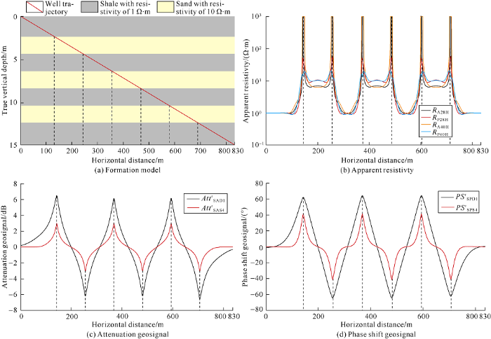
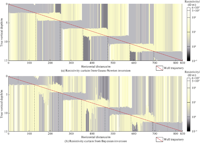
To validate the accuracy of dual-boundary model and inversion algorithm, a laminated sand-shale model was built as shown in Fig. 3(a), in which the sand and shale resistivity are 10.0 Ω·m and 1.0 Ω·m respectively. The upper most and lower most layers are 2.5 m thick each, while the layers in the middle are 2 m thick each. As the tool crossed beds at the relative dipping angle 89°, the corresponding apparent resistivity and amplitude ratio, and geosignals are shown in Fig. 3(b)-3(d). Clearly, sharp response changes occurred when the tool crossed the bed boundaries (see the dotted lines in fig. 3). Using Gauss-Newton optimization, the inverted 2D resistivity curtain shown in Fig. 4(a) was obtained. In the figure, the color of each pixel represents the value of the formation resistivity. Obviously, sudden resistivity changes took place when the tool passed the bed boundaries (see the dotted lines). In the resistivity curtain, the color of each point depicts the formation resistivity. Comparing Fig. 3(a) with Fig. 4(a) shows the boundaries corresponding to abrupt resistivity change points in Fig. 4 (see the dotted lines) are basically consistent with to the boundaries of the true model, indicating the Gauss-Newton algorithm is accurate and the dual-boundary inversion model is feasible. Note that although the remote bed boundaries may be unavailable, application of AEM in geosteering wouldn’t be affected. The inverted 2D resistivity curtain provides not only the upper/lower boundaries of the formation near the tool but also intuitive display of the formation structure. Fig. 4(b) shows the results from Bayesian inversion. Compared with Gauss-Newton inversion, Bayesian inversion is also capable of providing accurate boundary positions, for instance the dotted lines in Fig. 4(b). However, undesired resistivity perturbations occur at the bed boundary, indicating poorer stability of Bayesian inversion.
Fig. 3.
Responses of PeriScope in sand-shale laminates of 2.0 m thick each.
Fig. 4.
Dual-boundary inversion results of sand-shale laminates of 2.0 m thick each.
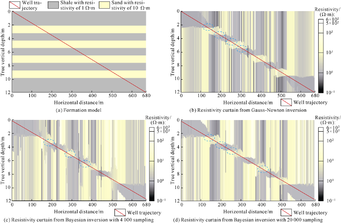
To demonstrate the applicability of dual-boundary inversion model in reservoirs with different thicknesses, a laminated sand/shale model was built. In this case, each bed is 1.0 m thick except for the upper most and lower most beds (2 m), and resistivities of sand and shale beds are 10.0 Ω·m and 1.0 Ω·m, respectively, as shown in Fig. 5(a). By performing the aforementioned inversion processing, the 2D resistivity curtains derived from Gauss-Newton and Bayesian inversion are shown in Fig. 5(b)-5(d). Obviously, the bed boundaries can be derived from both inversion methods, but the stability of inverted resistivity curtains reduces at the bed boundaries. To illustrate this, we circled the resistivity curtain near the bed boundaries where stronger perturbations are observed in the inversion result from Bayesian method. Comparing Fig. 4 and Fig. 5, we can conclude that: (1) dual-boundary inversion is applicable to formations more than 1.0 m thick, whereas the stability of inversion result reduces when the formation thickness is less than 1.0 m; (2) the result from Gauss-Newton inversion is slightly better than that from Bayesian inversion, and the precision of inverted parameters can be improved by increasing the iteration numbers.
Fig. 5.
Dual-boundary inversion results of sand-shale laminates of 1.0 m thick each.
3.2. Inversion with single-boundary model
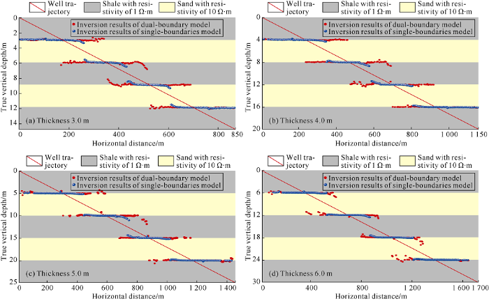
To verify the feasibility and accuracy of single-boundary inversion model, a formation model with five laminated sand/shale beds was constructed. Fig. 6 shows the corresponding estimated bed boundaries obtained from single-boundary and dual-boundary inversion models. The red and blue points represent the bed boundaries simulated by dual-boundary model and single-boundary model, respectively. For formations more than 3.0 m thick, as shown in Fig. 6a, single-boundary inversion can provide accurate boundary positions when the distance between the tool and approaching boundary is less than 0.9 m. Whereas the estimated distance may be smaller than its true value when the distance between the tool and adjacent boundary is larger than 0.9 m as the azimuth information is affected by multiple boundaries. Meanwhile, the accuracy and stability of inverted results improve with the increase of bed thickness. When the bed thickness is larger than 4.0 m, the estimated bed boundaries obtained from single-boundary and dual-boundary inversions are almost identical, as show in Fig. 6(b)-6(d). Generally, for beds more than 4.0 m thick, the single boundary inversion is able to provide accurate upper or lower boundaries less than 1.8 m away from the borehole, satisfying the needs of real-time geosteering. Note that inverted result of this section is obtained using the gradient method associated with single- boundary inversion model, and similar result can also be achieved by using Bayesian optimization method. The repetitive details are not given here.
Fig. 6.
Inversion results of estimated bed boundaries from single-boundary model and dual-boundary model.
3.3. Inversion with four-boundary model
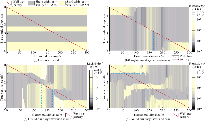
When the bed thickness is less than 1.0 m, there are multiple boundaries within the detection scope of the tool as a result, single-boundary or dual-boundary model may be oversimplified. In these cases, much more complicated multi-boundary model is needed to reveal the detailed distribution of formation structures around the borehole. Unfortunately, as the layers of inversion model increase, the inverted parameters increase and the corresponding local minima of the cost functional soar. The gradient method is no longer applicable and therefore Bayesian optimization method is adopted in this section. To illustrate the advantage of multi-boundary inversion, we built a formation model in which the middle layers were high resistivity beds of 0.6 m thick (the corresponding lateral distance varied from 135 m to 165 m along the well trajectory), as shown in Fig. 7(a). Fig. 7(b)-7(d) show the 2D resistivity curtains from single-boundary, dual boundary and four-boundary inversion models, respectively. From Fig. 7(b), we can see that the single-boundary inversion can only show the very top and bottom boundaries, but can’t show the thin beds since no sudden resistivity changes at lateral distance 135 m to 165 m are observed. When the dual-boundary inversion model is adopted, the nearest boundary can be determined when the tool is approaching or going away from the thin bed. Unfortunately, accurate upper and lower boundaries of the thin beds are still not identifiable when the tool lies in the thin beds. More specifically, sharp resistivity changes can be observed at 135 m and 165 m of the lateral distance, while the inverted resistivities at 135 and 165 m are not stable, as shown in Fig. 7(c). Fig. 7(d) shows the inverted resistivity curtain from four-boundary inversion. Similar to the dual- boundary inversion results, sharp resistivity changes are observed at 135 m and 165 m of lateral distance, whereas the resistivity distribution is much more stable at lateral distance of 135 and 165 m. The four-boundary inversion not only provides the upper and lower boundaries of current layer where the tool locates, but also gives the bed boundaries of further layers. Taking lateral distance 135 m for instance, we can get three boundaries with Tvd of 1.0 m, 2.3 m and 2.9 m (dash lines in Fig. 7d). We can conclude that the four-boundary inversion model can reconstruct the formation structure, so it can be used in fine evaluation of reservoir structure.
Fig. 7.
Four-boundary model and 2D resistivity curtains of Bayesian inversion.
3.4. Selection criteria of inversion model and inversion algorithm
Another concern in the selection of inversion model is the computation time. The inversion speed of Gauss-Newton method depends on the number of initial models and iterations, while the efficiency of Bayesian method is proportional to sampling number of MCMC. For single-boundary and dual- boundary inversion models, computation times of each measuring point in Gauss-Newton inversion are 0.3 s and 3.0 s, whereas Bayesian inversion requires 15 s and 60 s when 5 000 and 20 000 points are randomly sampled. By contrast, 500 s is needed for Bayesian algorithm with 100 000 sampling when the four-boundary inversion model is adopted. Considering the speed, precision and simplicity of inversion model, the selection criteria of inversion model and algorithm are showed in Table 1, where “A” and “N/A” depict “Applicable” and “Not-Applicable”, respectively.
Table 1 Selection criteria of inversion model and inversion algorithm.
| Thickness of target layer H/m | Single-boundary inversion model | Dual-boundary inversion model | Four-boundary inversion model | Gauss- Newton algorithm | Bayesian Algorithm |
|---|---|---|---|---|---|
| H>4.0 | A | N/A | N/A | A | N/A |
| 1.0<H<4.0 | N/A | A | N/A | A | N/A |
| H<1.0 | Non-appli- cab N/A e | N/A | A | N/A | A |
4. Case study
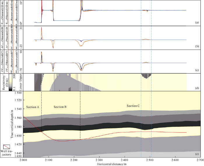
In this section, a horizontal well is presented to showcase the application of ARM in geosteering. As shown in Fig. 8, the horizontal well is divided into three sections. Section A corresponds to landing of the horizontal well. In section B, the well penetrated the lower boundary of target layer, then was adjusted and drilled back into the sand formation. In section C, the well trajectory was controlled in the payzone.
Fig. 8.
Real-time interpretation of LWD AEM data acquired in a horizontal well. (Different colors represent different layers in
If PS and Att geosignals are unavailable, the formation model is usually updated by correlating the horizontal well logs with an expected geological sequence defined by the offset well. Normally, resistivity and lithology curves are used in correlation. Using real-time well-correlation, relative positions between bed boundaries and well trajectory are readily obtained in section A and B. In section C (lateral distance: 2455-2535 m), abnormal declination, i.e. the interval between two blue dashed lines in Fig. 8(d), is observed in the apparent resistivity curves, indicating a conductive shoulder bed. However, due to the non-azimuthal property of apparent resistivity curves, it is difficult to accurately predict bed positions only using well correlation and the well could easily penetrate the target formation. By contrast, the amplitude of geosignal curve enlarges slightly in section C, indicating the tool is approaching the upper bed boundary. After inversion processing of AEM data, accurate positions of approaching boundaries can be derived. Thanks to the boundary information, the trajectory can be kept within the target layer and the distribution of formation structure is obtained.
5. Conclusions
In order to obtain the approaching bed boundaries in real-time, the complex 3D inversion of LWD AEM data is simplified into a series of 1D inversion problems using the dimensionality reduction scheme. For formations more than 4.0 m thick, the nearest boundary can be obtained by using the single-boundary inversion model. But when the bed thickness is between 1.0 m and 4.0 m, dual-boundary model instead of single-boundary one is needed to accurately estimate upper and lower boundaries of the formation and resistivity information of the formation. For the inversion of AEM data acquired in thin layers, especially when the layers are less than 1.0 m thick, the multi-boundary inversion model should be adopted. For single-boundary and dual-boundary inversion models, regularized Gauss-Newton method is good enough to extract formation boundaries in real time from AEM data, and the corresponding computation times of each recording point are 0.3 s and 3.0 s, respectively. For multi-boundary model, MCMC-based Bayesian algorithm can be used to interpret the formation boundaries in detail, and inversion time for each recording point is 500 s. Inversion results of actual field data show that nearby bed boundaries can be accurately picked using the optimal combination of inversion model and inversion algorithm. In addition, AEM has significantly reduced the uncertainty in the interpretation of conventional electromagnetic log data of horizontal wells, and has improved the capability of geosteering while drilling.
Nomenclature
Att—amplitude ratio, dB;
Att°—attenuation geosignal, dB;
Att°SAD1, Att°SAD4—attenuation geosignals with 243.84 cm (96 in) spacing operated at 100 kHz and 400 kHz, dB;
Att°SAS4—attenuation geosignal with 86.36 cm (34 in) spacing operated at 400 kHz, dB;
${{C}_{k}}\left( m \right),{\partial \text{C}}/{\partial m}\;$—cost function and its derivative;
${{d}^{\text{obs}}}$—observed data;
$F\left( m \right)$—L2 norm between observed data and simulated responses;
H—thickness of target layer, m;
Hup, Hdown—distances between record point and upper/lower bed boundaries, m;
Imag—imaginary part of a complex number;
J—Jacobian matrix;
k—iteration number;
$m$—model vector of interest;
${{\mathbf{m}}_{1}}$,${{\mathbf{m}}_{2}}$—arbitrary formation models;
N—number of bed boundaries;
$p\left( \mathbf{m} \right)$—priori probability density function;
$p\left( {{\mathbf{d}}^{\text{obs}}}|\mathbf{m} \right)$—likelihood probability density function;
$p\left( \mathbf{m}|{{\mathbf{d}}^{\text{obs}}} \right)$—posterior probability density function;
PS—phase shift, (°);
PS°—phase shift geosignal, (°);
PS°SPD1, PS°SPD4—phase shift geosignals with 243.84 cm (96 in)spacing operated at 100 kHz and 400 kHz, (°);
PS°SPS4—phase shift geosignals with 86.36 cm (34 in) spacing operated at 400 kHz, (°);
$q\left( {{\mathbf{m}}_{1}},{{\mathbf{m}}_{2}} \right)$—transition kernel function;
Real—real part of a complex number;
RA28H, RP28H—attenuation resistivity and phase shift resistivity with 2 MHz and 71.12 cm (28 in) spacing, Ω·m;
RA40H, RP40H—attenuation resistivity and phase shift resistivity with 2 MHz and 101.60 cm (40 in) spacing, Ω·m;
${{R}_{k}}\left( m \right)$—adaptive regularization term;
Rs1, Rs2—resistivities of shoulder beds in signal-boundary model, Ω·m;
Rt—formation resistivity where the tool lies in, Ω·m;
Rup, Rdown—equivalent resistivities of upper and lower adjacent beds in the dual-boundaries model, Ω·m;
$S\left( m \right)$—response from forward modeling m;
T—Transpose of a vector or matrix;
${{V}_{{{\text{R}}_{1}}}}$,${{V}_{{{\text{R}}_{2}}}}$—electric potentials of two coaxial receivers generated by coaxial transmitter, V;
${{V}_{{{\beta }_{1}}}}$,${{V}_{{{\beta }_{2}}}}$—electric potentials of tilted receiver at azimuthal angles ${{\beta }_{1}}$ and${{\beta }_{2}}$, V;
$\alpha \left( {{\mathbf{m}}_{1}},{{\mathbf{m}}_{2}} \right)$—acceptance probability function;
β—random number;
β1, β2—azimuthal angle of the drill collar during rotation, (°);
θ—relative angle between tool axis and formation, (°);
δ—initial value obtained by experiment.
Reference
Advancement and economic benefit of geosteering and well-placement technology
DOI:10.1190/tle34050524.1 URL [Cited within: 1]
New directional electromagnetic tool for proactive geosteering and accurate formation evaluation while drilling. New Orleans,
Investigation of eccentricity effects and depth of investigation of azimuthal resistivity LWD tools using 3D finite difference method
A new physical simulation system of drilling mud invasion in formation module
Three dimensional Born geometrical factor of multi-component induction logging in anisotropic media
Environment correction method of dual laterolog in directional well
2.5D forward and inverse modeling for interpreting low-frequency electromagnetic measurements
High fidelity real-time imaging with electromagnetic logging-while-drilling measurements
DOI:10.1109/TCI.2017.2670364 URL [Cited within: 1]
Bed-boundary effect removal to aid formation resistivity interpretation from LWD Propagation measurements at all relative dip angles. New Orleans,
Distance of detection for LWD deep and ultra-deep azimuthal resistivity tools. Oklahoma,
Real- time interpretation of formation structure from azimuthal EM measurements. Veracruz,
TORRES-VERDÍN C. Efficient 2D Bayesian inversion of borehole resistivity measurements
Characteristics of the sum of cross-components of triaxial induction logging tool in layered anisotropic formation
A general framework for constraint minimization for the inversion of electromagnetic measurements
DOI:10.2528/PIER03100702 URL [Cited within: 1]


