Introduction
Generally, the adjustment of oil well production is mainly based on the production law of the well,a series of production schemes were formulated by numerical simulation, and the final optimal scheme is sorted out through economic evaluation. But this method is large in workload, long in working period, and cannot ensure that the optimized result is the optimal solution. In recent years, domestic and foreign researchers have developed some reservoir production optimization techniques based on optimization methods successively, such as nonlinear programming[1,2], adjoint gradient method, and simultaneous perturbation stochastic approximation (SPSA) algorithm[3,4], which have achieved certain application effect. However, most of these methods mainly focus on the maximum economic benefit value of mathematics, but pay little attention to the actual production law of reservoirs, leading to inconsistency between some optimal results and the real production situation[5,6]. Therefore, in this study, taking the production law of reservoirs as the basic constraints, the optimal control mathematical model was established, the model was solved with the improved SPSA algorithm, and then the automatic optimization software for liquid production was made. To evaluate the practical application effect of the model, it is applied to optimize liquid production of reservoirs with strong natural aquifer in late development stage.
1. Liquid production optimization model
1.1. Establishment of mathematical model
With the rise of composite water cut, the production costs increase and economic benefits decrease gradually. It is necessary to carry out production optimization promptly, to obtain the maximum crude oil output at the lowest production costs, and reach the goal of controlling water cut and stabilizing oil production in the oilfield[7,8,9]. The liquid production optimal control method is to maximize the development benefit by optimizing the liquid production of wells in the oilfield. The net present value (NPV) is generally used to evaluate the economic benefits of oilfield development. The advantage of the net present value method is that it considers the economic status of the project throughout the calculation period, and the benefit of the project is represented in money and thus is very intuitive.
For reservoirs with strong natural aquifer, the production costs in the late development stage are mainly affected by factors such as operating cost and sewage treatment cost. Therefore, taking the operating cost and sewage treatment cost into consideration, an optimal objective function of the economic net present value was established:
For a real reservoir, due to the physical properties of the reservoir, the liquid production variation of the reservoir cannot exceed its actual supply ceiling. Meanwhile, due to the limit of gathering capacity and sewage treatment capacity, the maximum water production of the reservoir cannot exceed the gathering capacity and processing capacity. Therefore, constraints of the model should be added when optimizing the design, boundary constraints are common ones. The upper boundary needs to consider reservoir supply capacity and processing capacity of surface equipment. The lower boundary is usually set at zero, that is, shut down. Therefore, the constraints of the mathematical model for the liquid production optimization can be expressed as:
1.2. Improvement of mathematical model
Based on the above mathematical model, domestic and foreign researchers obtained optimal results of the control parameters by solving the most optimal value. However, this mathematic model does not consider the oil production decline and water displacement of oilfield, thus the oil production and water cut obtained through this optimization are sometimes inconsistent with the actual production. Therefore, in this study, the production law of reservoirs is taken as the basic constraints to improve the model of liquid production optimization and we establish the optimal control mathematical model constrained by the oilfield production law.
The oil production variation and water drive characteristics of reservoirs with strong natural aquifer are relatively stable in the late development stage. Under the same development mode, the current production pattern can be used to predict the production performance in the future. In this work, the Arps exponential decline curve and the A type water flooding characteristic curve were used to constrain the changes of oil production and water production. Among them, the expression of the Type A water drive curve is given by:
Transform Eq. 3 into Eq. 4 as:
Take the natural logarithm of both sides of Eq. 4 to get Eq. 5:
where $a={{a}_{0}}\ln 10$ $b={{b}_{0}}\ln 10$
After segmentation based on the adjustment interval, the water production at time i was obtained by using Eq. 5 as:
Considering the change of liquid production of the oilfield, the current oil production was divided into two parts, the oil production corresponding to naturally decline at the previous time and that to liquid production changes. Since the oil production in the late development stage of reservoir with strong natural aquifer is relatively stable, it is assumed that the decline rate of the liquid production is the same as the natural decline part. The production decline equation can be written as:
Substituting Eq. 6 and Eq. 7 into equation Eq. 1, an improved objective function is obtained (Eq. 8):
From Eq. 8, it can be seen that the optimization of liquid production is converted to the problem of getting the maximum value of the net present value under the constraint condition and optimizing the corresponding liquid production. The simultaneous perturbation stochastic approximation (SPSA) algorithm is often used to solve this type of optimization problem.
1.3. Solution of the mathematical model
The SPSA algorithm obtains the search direction by simultaneously perturbing the control variables, and the calculation is simple. Each iteration step only needs to calculate the objective function, and does not need to solve the real gradient, thus the computational complexity is effectively controlled.
where
$\Delta u=\left[ \begin{matrix} \Delta {{u}_{1}} & \Delta {{u}_{2}} & \cdots & \Delta {{u}_{N}} \\ \end{matrix} \right]=\left[ \begin{matrix} \Delta {{u}_{11}} & \Delta {{u}_{12}} & \cdots & \Delta {{u}_{1N}} \\ \Delta {{u}_{21}} & \Delta {{u}_{22}} & \cdots & \Delta {{u}_{2N}} \\ \vdots & \vdots & \ddots & \vdots \\ \Delta {{u}_{{{N}_{\text{u}}}1}} & \Delta {{u}_{{{N}_{\text{u}}}2}} & \cdots & \Delta {{u}_{{{N}_{\text{u}}}N}} \\ \end{matrix} \right]$
$\Delta J=\left[ \begin{matrix} \begin{align} & J\left( u+{{c}_{\text{k}}}\Delta {{u}_{1}} \right)-J\left( u \right) \\ & J\left( u+{{c}_{\text{k}}}\Delta {{u}_{2}} \right)-J\left( u \right) \\ \end{align} \\ \vdots \\ J\left( u+{{c}_{\text{k}}}\Delta {{u}_{N}} \right)-J\left( u \right) \\ \end{matrix} \right]$
The Eq. 9 is improved by reference of the standard SPSA gradient:
In Eq. 10, L is an N-dimensional upper triangular square matrix, and when L is a unit matrix, it is the standard SPSA algorithm. According to the SPSA convergence analysis:
It can be seen from Eq.11 that it still has the “uphill” characteristic. But the upper triangular matrix of L has an effect on the accuracy of the approximate gradient and needs to be adjusted to make the approximate gradient closer to the true gradient. Since the gradient is a vector, the closer the approximate gradient is to the real gradient, the smaller the angle between them is, the larger the corresponding cosine value is, and the cosine value is calculated as:
The true gradient in Eq. 12 is unknown. But the true gradient of each iteration step is deterministic. Therefore, we can choose the following equation as the optimization function of L to make sure that the angle between the calculated gradient and the real gradient of each iteration step is the smallest:
Firstly, the approximate gradient of the optimal control objective function is calculated. Then, according to the constraint conditions, the approximate gradient is processed with the projection gradient method, and then the iterative injection and production control variables are updated to obtain the optimal control variables:
2. Auto-optimization software for liquid production
Since the liquid production optimization model is complicated, it is very difficult to find the analytical solution by mathematical methods, and when using the simultaneous perturbation stochastic approximation algorithm to solve it, a large number of random disturbances are needed with large calculation workload. Therefore, according to the characteristics of the optimization model and the solution algorithm, the automatic optimization software for liquid production has been designed, significantly improving the calculation efficiency.
In the design of software, the solution process of the liquid production optimization model was strictly followed. First, the basic data required by the model was determined according to the actual data of the oilfield, such as oil production, water production, crude oil price, waste treatment cost, etc. Second, by using Type A water drive curve and the decline equation, the parameters a, b, d, etc. of the model were matched. And then, the SPSA algorithm was used to solve the optimization model of the liquid production. Finally, the optimal adjustment parameters of the liquid production were worked out.
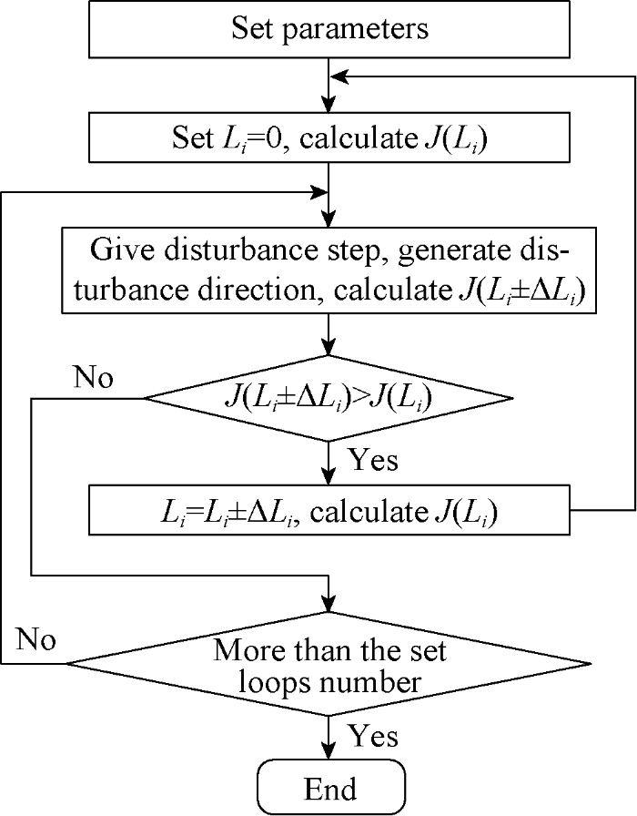
The main calculation process solving the liquid production optimization model by SPSA algorithm is shown in Fig. 1: (1) Set the basic parameters of the crude oil price, oil production, and decline rate according to the actual situation. (2) Set the liquid production change at zero at each time point initially and calculate the economic net present value J (Li). (3) Give the maximum value of the liquid production change (distur-bance step) at each time point, and use the random function to generate the disturbance direction, and calculate the economic net present value of the disturbance, J(Li±ΔLi). (4) Judge the relationship between J(Li±ΔLi) and J (Li), if J(Li±ΔLi) is greater than J (Li), the liquid production change is set as Li= Li±ΔLi and repeat steps (2), (3) and (4). If J(Li±ΔLi) is less than or equal to J (Li), the number of loops is judged. (5) If the number of loops exceeds the designed value, the optimization is ended. If not, repeat steps (3), (4), and (5).
Fig. 1.
Fig. 1.
Flow chart of automatic optimization of liquid production.
3. Application example
The D oilfield is located in the tropical rainforest of Ecuador in South America. Its main reservoir M1 is a tidal-controlled estuary sediment, with a porosity of 20% to 32% (25% on average) and a permeability of (1 000-8 000)×10-3 μm2 (4000×10-3 μm2 on average), strong edge-bottom water, and difference between reservoir pressure and saturation pressure of 18.2 to 19.4 MPa, belonging to medium-high porosity, medium-high permeability, strong edge-bottom water, low amplitude, tectonic-lithological sandstone reservoir. Put into production in March 1978, the reservoir is mainly driven by the edge-bottom water, with spot water injection as assistance means to supplement energy and irregular well pattern. After 40 years of development, it has a composite water cut of 96.5% and is in the late stage of development. Limited by the geological conditions of the reservoir and the relevant laws and regulations of Ecuador, it is difficult to tap the remaining oil through workover. Furthermore, the operation cost is high, and the economic benefits are marginal. In order to maximize the benefits in the late stage of oilfield development, the mathematical model of automatic optimization of liquid production was established and solved with the optimal control theory, realizing the automatic optimization of the liquid production of each well in the oilfield.
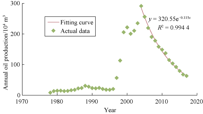
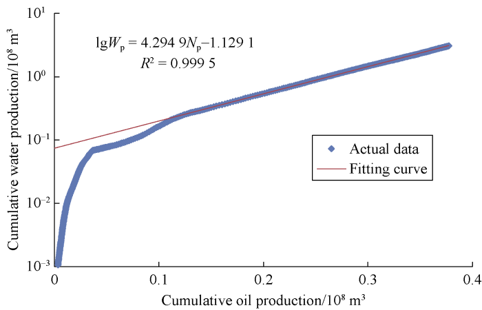
The production decline curve and water flooding characteristic curve were matched by using the oil production and water production data of the reservoir. Because the characteristics of production decline and water flooding are relatively stable, the correlation coefficients of the fitted results are both above 0.99 (Figs. 2 and 3).
Fig. 2.
Fig. 2.
Production decline curve of D reservoir.
Fig. 3.
Fig. 3.
Water flooding characteristic curve of D reservoir.
According to the fitting results, the basic parameters a, b, and d related to the model calculated are -1.1291, 4.2949, 0.1150, respectively. Meanwhile, according to the actual situation of the reservoir, the price of crude oil was set at 305.5 dollars/m3, the operation cost was 91.7 dollars/m3, and the waste treatment cost was 1.8 dollars/m3. After considering boundary constraints on the pipeline gathering capacity and waste treatment capacity of the D oilfield, the improved liquid production optimization model was used to optimize and predict the development indexes.
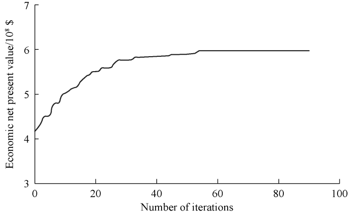
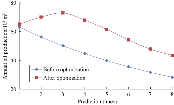
Through continuous automatic optimization, the economic net present value of the scheme gradually approached the best economic net present value of 5.98×10⁸ US dollars from 4.15×10⁸ US dollars. The economic net present value changing curve during the automatic optimization process is shown in Fig. 4. According to the optimization results (Figs. 5 to 7), the annual oil production will increase during the period when liquid production increases, while the annual oil production will decrease significantly during period when the liquid is kept stable, and the decline rate is the same as the actual decline rate of the D reservoir. The water cut during the forecast period will increase steadily. Comparing the data before and after optimization, it can be seen that after optimization, the liquid production and oil production both increase significantly, but the water cut change is basically the same. The reasons for this result are mainly: (1) The reservoir is in the late stage of development, and the oil is displaced mainly by water flooding, so the water cut is less affected by the liquid production change. (2) Most of the water produced is reinjected back into formation at lower cost, so the economic benefits are not sensitive to the increase in water production.
Fig. 4.
Fig. 4.
Economic net present value changing curve during automatic optimization.
Fig. 5.
Fig. 5.
Annual oil production curves before and after optimiztion.
Fig. 6.
Fig. 6.
Annual liquid production curves before and after optimization.
Fig. 7.
Fig. 7.
Annual water cut curves before and after optimization.
4. Optimization method comparison
Widely used in the formulation of oilfield development and adjustment schemes in China and overseas, the numerical simulation method has authority and general applicability, therefore, the method presented in this paper is compared with the numerical simulation method (Table 1).
Table 1 Comparison of numerical simulation and automatic optimization of liquid production
| Method | Single calculation time/min | Time needed to get optimization result/h | Objectivity | Optimization process |
|---|---|---|---|---|
| Numerical Simulation | 480 | 168 | Personal experience has a greater impact | Need to repeat the scheme, manual selection |
| Automatic optimization of liquid production | 5 | 2 | Not affected by personal experience | Automatic optimization |
The calculation process of the numerical simulation method is complicated, it is necessary to establish a geological model, prepare a numerical simulation model, and perform history matching. According to the possible range of liquid production, a large number of liquid production adjustment schemes are designed, and then prediction and comparison are carried out. It often has to go through multiple round of optimization to get the final optimization adjustment parameters. Thus, the numerical simulation method has low calculation efficiency and long calculation cycle, and is greatly affected by the experience of the simulation operator. Moreover, it can only compare the given plans, and cannot automatically optimize.
The method presented in this paper is relatively simple, and doesn’t need to establish a complex geological model or perform repeated history matching. After the initial values are set, it can automatically optimize, and the calculation process is not affected by human factors. Its calculation is high in efficiency and takes less time.
5. Conclusions
The traditional optimization control model only considers the mathematical maximum of the model but does not fully consider the law of oil production. Aiming at this problem, the production law of reservoirs with strong natural aquifer in late development period is taken as the basic constraint condition, and the optimal control mathematical model under the constraint of production law is established, avoiding the problem that the prediction result is inconsistent with the production law.
The SPSA algorithm was used to solve the model, and the automatic optimization software for liquid production has been made. The software was applied to the development and production stage of D reservoir in Ecuador, South America, and realizing automatic optimization of liquid production in the late stage of oilfield development.
Comparing the optimization process of liquid production optimization model with numerical simulation method, it is found that the liquid production optimization model has higher calculation efficiency, shorter calculation cycle and automatic optimization, which can meet the automatic optimization of liquid production in the late stage of oilfield development and also provide a reference for similar oil reservoirs.
Nomenclature
a0, b0—type A water flooding curve fitting constants;
ck—disturbance step;
Cmi—the operating cost at time i, dollars/m3;
Cwi—waste water treatment cost at time i, dollars/m3;
d—production decline rate, f;
fw,i-1—water content of the oil field at time i-1, f;
F(L)—optimization function of approximate gradient;
g—true gradient;
$\hat{g}$—approximate gradient;
Ic—the benchmark rate of return, f;
J—the economic net present value, dollars;
l—the iteration number;
Li—the amount of liquid produced by the oil field at time i, m3/a;
N—disturbance number;
Np—cumulative oil production, m3;
Np,i-1—the cumulative oil production of the oil field at time i-1, m3;
Nu—control variable dimension;
Poi—the price of crude oil at time i, dollars/m3;
Qoi—the oil production of the oil field at time i, m3/a;
Qwi—the water production of the oil field at time i, m3/a;
t—total time, a;
u—control variable;
ui—control variable of oil field at time i;
udi—lower constraint boundary of control variable;
uui—upper constraint boundary of control variable;
Wp—cumulative water production, m3;
θ—the angle between the approximate gradient and the true gradient, (°);
ΔLi—the increment of the liquid production at the time i, m3/a;
Δti—the time interval corresponding to the time i, a;
Δupg—disturbance interval of control variable u, p=1, 2,…, Nu,q=1, 2,…, N3;
α—disturbance coefficient in the lth iteration of control variables.
Reference
Multi-objective programming model of oilfield production based on different priority
An integrated mathematical programming approach for the design and optimization of offshore fields
The application of simultaneous perturbation stochastic approximation method in production optimization of polymer flooding
Production optimization of oil reservoirs based on an improved simultaneous perturbation stochastic approximation algorithm
A goal programming model for optimizing output of an oilfield
Improvement on the study of output optimization model of oilfields
Dynamic optimization of waterflooding with smart wells using optimal control theory
Water-cut rising mechanism and optimized water injection technology for deepwater turbidite sandstone oilfield: A case study of AKPO Oilfield in Niger Delta Basin, West Africa
New water drive characteristic curves at ultra-high water cut stage
Reservoir production optimization using an upgraded perturbation gradient approximation algorithm
Improved reservoir management through optimal control and continuous model updating
Closed-loop reservoir management on the Brugge test case


