China National Science and Technology Major Project. 2016ZX05023
Abstract
To resolve the issue of design for multi-stage and multi-cluster fracturing in multi-zone reservoirs, a new efficient algorithm for the planar 3D multi-fracture propagation model was proposed. The model considers fluid flow in the wellbore-perforation-fracture system and fluid leak-off into the rock matrix, and uses a 3D boundary integral equation to describe the solid deformation. The solid-fluid coupling equation is solved by an explicit integration algorithm, and the fracture front is determined by the uniform tip asymptotic solutions and shortest path algorithm. The accuracy of the algorithm is verified by the analytical solution of radial fracture, results of the implicit level set algorithm, and results of organic glass fracturing experiment. Compared with the implicit level set algorithm (ILSA), the new algorithm is much higher in computation speed. The numerical case study is conducted based on a horizontal well in shale gas formation of Zhejiang oilfield. The impact of stress heterogeneity among multiple clusters and perforation number distribution on multi-fracture growth and fluid distribution among multiple fractures are analyzed by numerical simulation. The results show that reducing perforation number in each cluster can counteract the effect of stress contrast among perforation clusters. Adjusting perforation number in each cluster can promote uniform flux among clusters, and the perforation number difference should better be 1-2 among clusters. Increasing perforation number in the cluster with high in situ stress is conducive to uniform fluid partitioning. However, uniform fluid partitioning is not equivalent to uniform fracture geometry. The fracture geometry is controlled by the stress interference and horizontal principal stress profile jointly.
Keywords:horizontal well
;
multi-stage fracturing
;
multi-fracture growth
;
3D boundary element
;
planar stress heterogeneity
;
perforation optimization
CHEN Ming, ZHANG Shicheng, XU Yun, MA Xinfang, ZOU Yushi. A numerical method for simulating planar 3D multi-fracture propagation in multi-stage fracturing of horizontal wells. [J], 2020, 47(1): 171-183 doi:10.1016/S1876-3804(20)60016-7
Introduction
Multi-stage and multi-cluster fracturing in horizontal wells is a crucial technology to develop unconventional oil and gas[1,2,3]. To increase the stimulated reservoir volume, many north American petroleum companies have been trying to reduce well spacing and fracture spacing in recent years[4]. However, field measurements by using distributed temperature sensing and distributed acoustic sensing show that uneven distribution of injected fluid occurs for closely spaced fractures, which is commonly dependent on the perforation design and distribution of in-situ stress among multiple fractures[5]. Therefore, an efficient algorithm for modeling multi-fracture growth considering the coupled system of “wellbore-perforation-fracture” is essential to improve the uniform growth of multiple fractures.
The classical fracture model can be 2D, pseudo-3D, planar 3D, and fully 3D[6]. The 2D models are PKN (Perkins-Kern-Nordgren) model and KGD (Khristianovich- Geertsma-Daneshy), suitable for a single fracture with constant height. Pseudo-3D models include lumped model and PKN cell-based model. The lumped model assumes that the fracture is comprised of two half-ellipses joined at their centers in the fracture length direction, in which only requires long axis and short axis to determine its shape[7]. The cell-based P3D model uses the equilibrium height analytical solution to solve the fracture height in each element, and fluid flow is in the direction of fracture length. The computational burden is much reduced by this method, but the fracture height prediction may be erroneous when fracture height is unconfined by larger stress barriers[8]. The cell-based P3D model has been applied to the multi-fracture simulation by Kresse et al.[9]. Zhao et al. [10] also proposed a multi-fracture P3D model and established an optimization method for perforation design. Since interaction stress among multiple fractures is calculated based on a 2D method in P3D model, the multi-fracture height growth maybe not really accurate[11]. Therefore, researchers, such as Advani[12], Barree et al.[13], proposed a planar 3D model to simulate fracture propagation. PL3D model uses a 3D elasticity equation to solve rock deformation and determine fracture geometry by fracture moving boundaries. Peirce et al.[14] proposed an implicit level set algorithm to simulate planar 3D fracture by introducing the tip analytical solutions. Then Dontsov et al.[15] derived a universal tip analytical solution and used it in the implicit level set algorithm[16]. Chen et al.[17] simulated the multi-fracture geometry by using the implicit level set algorithm. To describe the fracture twist, Carter et al.[18] proposed a fully 3D model. The fully 3D model is time-consuming even with today’s powerful computational resources. Xu et al.[19] developed a nonplanar multi-fracture simulator, called “FrackOptima,” in which the multi-fracture is assumed vertical 3D. The commercial application of fully 3D model is still unreported since the computational burden is extremely heavy and the unresolved physical questions about the propagation of fully 3D fractures[20]. Additionally, a complex hydraulic fracture model is presented recently to simulate fracture propagation in naturally-fractured reservoirs[21,22,23,24]. As our focus is the multi- fracture growth in the coupled system of “wellbore-perforation-fracture”, the interaction of hydraulic fracture with natural fractures are not considered in the present model.
From the analysis of the present fracture models above mentioned, PL3D model is most useful and feasible considering its accuracy and efficiency. The widely accepted algorithm is an implicit level set algorithm (ILSA) proposed by Peirce et al.[14] and Dontsov et al.[16]. This algorithm uses an implicit method to solve the coupling solid-fluid equation with multi- fracture propagation, and the fracture front is determined by an implicit level set method. The implicit method is unconditionally stable but requires to solve a large system of nonlinear equations, which is time-consuming. Particularly, the dense matrix from the boundary integral equation worsens the computational burden. Furthermore, for the case of proppant transport and fracture closure, more nonlinear constraints are added to the nonlinear equations, which further makes it more challenging to be solved. Besides, the field application of the implicit level set algorithm is less reported and perforation friction is not considered in its recent published version[25].
In the study, we proposed a new algorithm for solving the PL3D model, where an explicit integration method is adopted to solve the stiff equations of the coupled solid-fluid system. The fracture fronts are located by a shortest path algorithm with the tip analytical solutions. The accuracy and efficiency of the model were validated by comparing with the analytical solution[26], experimental results of CSIRO (Commonwealth Scientific and Industrial Research Organization)[27], and implicit level set algorithm (ILSA)[16,28]. Numerical simulations are performed on a multi-cluster fracturing treatment in a horizontal well in Zhejiang Oilfield. Then the influence of heterogeneous in-situ stresses among multiple fractures and distribution of perforations is discussed.
1. Mathematical model
1.1. Assumptions
The geometry of the present PL3D model is presented in Fig. 1. The number of clusters in a single stage is nf; each cluster is labeled as k. There are four physical processes involved in multi-fracture growth: fluid flow in the wellbore and multiple fractures; rock deformation under the net pressure, fluid leak-off into the formation; and the rock breakage at the fracture fronts. The assumptions adopted in the study are the same as those used in the implicit level set algorithm[14], listed as follows. The fluid leak-off obeys Carter model; The lag between fracture front and the fluid front is neglected, and the fracture propagation direction is perpendicular to the direction of the minimum principal horizontal stress. Previous researches[29,30,31], such as Bunger et al., Xu et al., and Tang, show that fracture curving is not significant, especially for reservoirs with high-stress contrast in Sichuan Basin, China, so the planar hydraulic fracture is a reasonable assumption.
Solid elasticity equation is used to describe the fracture width distribution under the internal fluid pressure and in-situ stress. Based on the fundamental solution in an infinite elastic media, we can obtain the boundary integral equation to describe the solid deformation[14] :
$p-{{\sigma }_{\text{h}}}=\int_{A\left( t \right)}{{{C}_{\text{g}}}\left( x-{x}',y-{y}',z-{z}' \right)w}\text{d}A$
1.2.2. Fluid flow equation
(1) Fluid flow in the wellbore. Since the effect of flow friction on flow rate distribution between the closely spaced fractures is relatively small[32], the flow friction in the wellbore can be neglected. Thus the bottom hole pressure of each fracture can be expressed as:
The range satisfying the solution of LEFMs is very small, so only very fine mesh can capture the condition described in equation (8). To capture the tip condition under a coarse mesh, we use the tip analytical solution to locate the fracture front[16]. Fig. 2 shows application range of the LEFMs and analytical solutions.
The critical fracture width at the fracture front is dependent on the fracture propagation rate, propagation length, fracture toughness, elasticity modulus, and leak-off coefficient. When propagating, the fracture front satisfies the following equation:
Equation (11) is a nonlinear equation that determines the fracture growth rate, mesh size, and critical fracture width. As the range of δ is very small, an approximate method proposed by Dontsov is used to solve simplified equation (11), which has an error of less than 0.3%[15]. The detailed solution is as follows.
(1) Let δ=0, a zero-order approximation to equation (11) can be obtained:
Equation (14) governs the tip growth rate, the critical fracture width, and the propagation step size. Since the range satisfies equation (14) is much larger, a coarse mesh can be adopted to improve computational efficiency.
2. Numerical methods
2.1. Mesh system
A fixed 2D grid is used to discretize the footprint of the fracture. Four kinds of elements are defined: injection element, channel element, tip element, and non-activated element, as shown in Fig. 3. The element type is updated in each time step by checking the propagation condition for each tip element. The fracture width and pressure in each element are located at the center of each element, and the flow rate is located at the edge of each element.
Constant displacement discontinuity method[34] is used to discretize the solid equation. The width of the element center point is approximated as the element width, then the discretized form of boundary integral equation is expressed as:
${{p}_{i,j,h}}\left( t \right)={{\sigma }_{\text{h}}}\left( x,y,z \right)+\sum\limits_{m,n,r}{{{C}_{i-m,j-n,h-r}}{{w}_{m,n,r}}\left( t \right)}$
Rewrite equation (15) into a matrix form:
$p={{\sigma }_{\text{h}}}+Cw$
2.2.2. Discretized flow equation
(1) Discretization of flow equation in the fracture. The governing equation (7) is discretized in space to get the first-order differential equation (ODE) of the flow equation:
$\frac{\text{d}w}{\text{d}t}=\left[ \theta A\left( w \right)p+\left( 1-\theta \right)A\left( {{w}_{0}} \right){{p}_{0}} \right]+S$
Where the components of A(w)p and S are respectively:
The equation (17) is an explicit format when θ=0, instead, it is an implicit format when θ=1. As equation (17) is a stiff equation, the explicit format should satisfy the Courant-Friedrichs-Lewy (CFL) condition to ensure the stable calculation, so most researchers use the implicit method to solve equation (17)[6,7]. The implicit algorithm is stable unconditionally and doesn’t need CFL conditions, but it has some disadvantages as well: First, the implicit algorithm needs to solve linear equations iteratively by the Newton-Raphson method or fixed- point method[6,7]. As the influence coefficient matrix C is dense, a direct method is often used to solve. The computation of the direct method is dependent on the number of elements, when the number of elements increases, the computation is huge and time-consuming. Although some preconditions can reduce the computation to some extent, the computational load is still huge when the number of elements is larger[35]. Second, more constraints for the coupled fluid-solid equation are included when nonlinear problems such as proppant transport or fracture closure are considered, which makes it more difficult to solve the equation by implicit algorithm[35]. Third, to ensure calculation precision, the time step for the implicit algorithm shouldn’t be too large[7, 28].
Since the implicit algorithm still has computation difficulty and high time consumption, we use the explicit algorithm to solve the stiff equation (17). To improve the computational efficiency, a stabilized Runge-Kutta-Legendre (RKL) method is adopted to solve equation (17). Multiple steps integration was used based on the recursive formula of Legendre polynomials. CFL time step can be extended remarkably to reduce computation load and enhance computation efficiency.
Since the absolute value of Legendre recursive polynomials is less than 1, S internal steps were used for a single integration. The second-order accurate S-stage RKL scheme can be found in reference [36]. The stable time-step for the S-stage RKL is:
For the fracture growth, under the prerequisite of ensuring stability, the computation precision should be considered when selecting time step, so the time-step in S-stage RKL is determined as:
ε is a relaxation factor, 0<ε≤1. In our simulations, the relaxation factor is 0.8. However, when in-situ stress heterogeneity is considered, the relaxation factor should be smaller to avoid overshoots as the fracture acceleration may be possible in case of fracture growing into a lower in-situ layer.
2.4. Tip location
Peirce et al.[14] and Dontsov et al.[16] calculated the position and width of fracture tip by analytical solutions of the activated elements next to fracture tip elements. In this study, we use the critical fracture width and fracture propagation velocity in the non-activated elements at the tip to locate the fracture front. In each time step, the associated non-activated elements adjacent to the tip elements are updated as new tip elements when the propagation criterion is satisfied. The opening time of each element is determined by the shortest path algorithm. Note that the fracture front is reconstructed by activating the grid[13].
As shown in Fig. 4, For the non-activated element a, the adjacent elements are b, c, d, e. The opening time of element a is determined by the shortest path algorithm:
Before the non-activated element is opened, its current opening time is infinite. For example, if the elements b, c, and d are non-activated, and e is an activated element, then the opening time of the element a is:
When vea satisfies the propagation criterion in equation (11), the element a becomes a new tip element.
2.5. Algorithm
The algorithm for the planar 3D multi-fracture model is as follows.
(1) Set input injection time tf, rock mechanical parameters, pumping schedule, fluid properties, and in-situ stress distribution, etc.;
(2) Let α=0, t=t0, then calculate the initial fracture width w0 and pressure p0;
(3) Let α=α+1, t=t+Δt, then the fracture width wα and pressure pα of the activated element now can be obtained by solving equation (22). This procedure ends when t>tf.
(4) The flow rate distribution in clusters is obtained by solving equation (20) with the Newton-Raphson method.
(5) Calculate the number of elements to be activated potentially at the current time step. The critical fracture width of each element to be activated is calculated based on equation (11). When the calculated fracture width reaches the critical value from equation (11), the associated non-activated element can be updated as a new tip element.
(6) All the potential elements are checked and the status of all the elements are updated. The new tip elements and adjacent non-activated elements are determined, then return to step (3).
The algorithm contains three main parts: fluid partition among multiple fractures, coupled solid-fluid equations, and fracture front updating. The fluid partition among multiple fractures is solved by a Newton-Raphson method, which is second-order accurate. The RKL method for the coupled solid-fluid system is second-order accurate and stable[36]. The region satisfying the tip asymptotical solutions is about 10% of fracture length, while the region satisfying the LEFM region is only 0.1%-1.0% of fracture length. Thus a relatively coarse mesh can be adopted by using the tip asymptotical solutions[37], which reduces the computational burden. The three parts of the algorithm all satisfy convergence and stability; hence, the algorithm is reasonable theoretically.
3. Validation and efficiency comparison
3.1. Model accuracy
3.1.1. Comparison with analytical solution of penny-shaped fracture
We first validated the model against analytical solutions. The HF is penny-shaped when the inter-layer stress difference is zero. Since the HF usually grows in a viscosity-dominated way of energy dissipation for field cases, we used the viscosity-dominated penny-shaped fracture to verify our model.
The basic inputs for the validation case are Qt=5 m3/min, μ=5 mPa∙s, E=30 GPa, v=0.2, KIc=0.2 MPa·m1/2, Cl=0, tf=10 min. The characteristic time for the propagation of a penny- shaped HF is[30]
When the injection time is far less than the characteristic time, the HF grows in a viscosity-dominated regime; while the HF grows in a toughness-dominated regime when the injection time is much larger than tc. The characteristic time in this validation case is 3.30×10⁹ min, which is far more than the injection time (10 min), indicating the HF growth is viscosity-dominated. The fracture radius and inlet width of a viscosity-dominated penny-shaped HF are respectively[30]:
The dimension of the element in this validation case is 2.5 m×2.5 m. The results are plotted in Fig. 5. The numerical results agree with the analytical solutions quite well (Fig. 5), suggesting the algorithm can capture the fracture growth of a penny-shaped fracture accurately.
Fig. 5.
Comparison of results from the algorithm presented in this paper and analytical solutions of the penny-shaped fracture.
3.1.2. Comparison with the implicit level set algorithm
To further test the accuracy of the algorithm, we consider a case in which multi-layer confining stresses are applied in a permeable formation with fluid leak-off. Dontsov and Peirce[16] simulate this case by using their ILSA simulator. Three different confining stresses are applied, as shown in Fig. 6a. The other basic inputs for this case[16] is E=9.5 GPa, v=0.2, μ=0.1 Pa•s, Qt=0.01 m3/s, KIc=1 MPa·m1/2, and Clv=2.065× 10⁻⁶ m/s1/2.
Fig. 6.
Fracture propagation profiles with multi-layer confining stresses and fluid leak-off and comparison of fracture geometries with results from Dontsov et al.[16].
Fig. 6b shows the comparison between the fracture width profile calculated by our algorithm and the fracture geometry from reference [16]. It can be seen that the fracture boundary from our algorithm matches well with the ILSA’s result in reference [16], proving our algorithm can solve fracture propagation accurately in the case with fluid leak-off.
3.2. Efficiency comparison
This validation case was the fracturing experiment of PMMA in CSIRO[27]. PMMA is linearly elastic and homogeneous, and the fracture boundary can be monitored as its transparency. The basic parameters in the experiment are listed as follows: Three-layer confining stresses are applied, as shown in Fig. 7. The fluid viscosity is 30 Pa·s, Young’s modulus is 3.3 GPa, and Poisson’s ratio is 0.4. A variable injection rate is used in the experiment[27]. Fig. 8 shows the comparison of fracture geometry between the numerical result and experimental result at 665 s. The numerical results agree well with the experimental results, which further demonstrates that the accuracy of our numerical model and makes the efficiency comparison reasonable.
Fig. 8.
Comparison of experimental results from our algorithm and CSIRO.
Zia et al.[28] simulated the fracture growth of the experi-mental work in reference [27] by using ILSA and evaluated the computational efficiency. To determine the computational efficiency, we use a same-size mesh as that in reference [28] and the same process that is Intel(R) Core(TM) i7-5600 CPU@2.60GHz. The ILSA simulator in reference [28] used a Python code, while our algorithm uses MATLAB, which have similar execution efficiency. The computation time was within 300 s for the RKL of 25, 50, and 75 stages of integration. Particularly, the CPU time for RKL of 75 internal stages was 73 s, which is much less than the CPU time of 619 s by using ILSA in reference [28]. Apparently, our algorithm is much higher in computation efficiency.
4. Case studies
Numerical simulations were conducted based on the data of the horizontal well YS112H4-1 in the shale gas demonstration region of Zhaotong in the Zhejiang Oil field. The pay zone of Well YS112H4-1 is lower Silurian Longmaxi Formation. This well was designed to be fractured at multi-stage at a small fracture spacing of 10 m and an injection rate of 14 m3/min. The fracturing fluid was FAB-2 slick-water with a density of 1016 kg/m3, viscosity of 2 mPa·s. The reservoir is 34 m thick and has a horizontal stress difference of 17.0-19.5 MPa. The reservoir rock has an elasticity modulus of 35.7 GPa, Poisson’s ratio of 0.27, and fracture toughness of 1.0 MPa·m1/2. The reservoir has a matrix permeability of 1.0×10⁻⁷ μm2, so the fluid leak-off into formation can be neglected. The pay zone is between layers with confining stress, and its minimum horizontal principal stress profile is shown in Fig. 9. In the figure, the position of the perforations is z=0. The perforations are 12 mm in diameter and 0.7 of the correction coefficient.
Fig. 9.
Schematic diagram of in-situ stress profile and multi- clusters of perforations.
As many studies[38-40] have discussed the relationship of perforation diameter and clusters number with fluid rates in multiple clusters, this study focuses on the effect of stress distribution, perforation number, and distribution of perforations on flow rate and fracture propagation.
4.1. Effect of the in-situ stress distribution on fluid distribution in the clusters
4.1.1. Homogenous in-situ stress
We first examined the case of homogeneous in-situ stress on the plane; namely, all clusters had the same minimum horizontal principal stress of 60 MPa. In this case, the perforation friction and stress interference control the fluid distribution in multiple clusters.
Fig. 10 shows that all the clusters can be initiated and propagated when there are 4, 8, and 16 perforations in each cluster and the perforation clusters are homogeneous in stress distribution. The fluid volumes into all the clusters are similar when each cluster has 4 or 8 perforations. The fluid volume into the exterior cluster is 1.24 times than that in the inner fracture when each cluster has 16 perforations. Therefore, it can be seen that the more perforations in each cluster, the larger the difference of fluid volumes between clusters.
Fig. 10.
Fluid volume distribution in clusters under homogeneous in-situ stress distribution.
As shown in Fig. 11, the fractures of all clusters are similar in length when the number of perforations is 4 or 8 in each cluster. Whereas the exterior fracture is 330 in half-length, approximately 1.24 times longer than the inner fracture (265 m) when the number of perforations in each cluster is 16. Moreover, the fracture tends to grow upward due to the relatively smaller in-situ stress in the upper zone. The fracture height of the inner fracture near the wellbore is larger than that of the exterior fracture, indicating the stress interference is more significant near the wellbore. Under the compressive stress induced by nearby fractures, the inner fractures tend to grow in a vertical direction.
Fig. 11.
Geometries of fractures under homogeneous in-situ stress distribution.
4.1.2. Effect of heterogeneous in-situ stress
Set the σh for clusters 1 to 5 in the pay zone were 62, 60, 60, 60, and 60 MPa, respectively, namely, the in-situ stress in cluster 1 was 2 MPa larger than the other clusters.
Fig. 12 shows that the fluid volume into the high-stress cluster is less than that into the other clusters, but all the clusters filled with fluid when the number of perforations per cluster is 4 or 8. But the high-stress cluster is not initiated when the number of perforations per cluster is 16, suggesting that the perforation friction of 16 holes per cluster is not able to counterbalance the in-situ stress difference of 2 MPa. In contrast, when there are 8 perforations in each cluster, fluid can enter all the clusters, and when there is 4 perforations per cluster, fluid volumes into all clusters are similar.
Fig. 12.
Fluid volumes of different clusters in the case of heterogeneous distribution of in-situ stresses.
Although the fracture of cluster 1 is less suppressed by interaction stress from other fractures, it will be un-activated when the minimum horizontal principal stress is 2 MPa larger than other clusters. Hence, the heterogeneous in-situ stress among clusters has a stronger effect on the fluid distribution among clusters than stress interaction. Therefore, understanding the distribution of in-situ stress in the pay zone is important for the design of multi-cluster fracturing and flow-restricted.
Fig. 13 shows that when the number of perforations is 4 or 8, although the fluid volumes into the clusters don’t differ much, as the in-situ stress is smaller in the upper part of the zone than the lower part, and the growth of HF1 is influenced by interaction stress, the HF1 tends to propagate towards the upper part of the zone, resulting in overgrowth of the fracture height. Clearly, the fracture propagation is controlled by interlayer stress profile and stress interference jointly. The fracture would grow along the path with the smallest resistance, the fracture would grow vertically when the stress interference is stronger than the inter-layer stress difference. Affected by interlayer stress distribution and stress interference, the fractures in the high-stress zone may change in shape, impairing fracturing effectiveness. This means that the production and fluid intake of a cluster may be inconsistent. This kind of situation is hard to be discovered from downhole temperature or acoustic monitoring. Therefore, the distribution of in-situ stress among clusters should be carefully analyzed during fracturing design, and the intervals with similar in-situ stress should be designed as one stage.
Fig. 13.
The fracture geometry in the case of heterogeneous distribution of in-situ stresses.
4.2. Effect of perforation number distribution on fluid distribution
4.2.1. Homogeneous in-situ stress among clusters
Cramer et al.[41] found that not all the perforations were active during the injection process by down hole observation due to differences in perforation quality and phase. Thus we analyzed the effect of non-uniform distribution of perforations on fluid distribution. Three kinds of perforation designs were investigated. The perforation numbers of cluster 1 to cluster 5 were: (1) 8, 9, 8, 8, 8; (2) 8, 10, 8, 8, 8; (3) 8, 11, 8, 8, 8. The minimum horizontal principal stresses of all the clusters are the same as 60 MPa.
Fig. 14 shows that HF2 takes most fluid when 1-3 perforations are added in HF2. Also, the injected fluid volume becomes larger with the number of added perforation in HF2. The fluid volume ratio in HF2 is 21.5%, 23.3%, and 25.0%, when adding 1, 2, and 3 perforations, respectively. For the three perforation design, adding 3 more perforations in HF2 is not recommended as it causes the HF2 receiving much more fluid. Fig. 15 shows that adding too many perforations in a specific cluster may result in over-correction, which may aggravate the nonuniformity of multiple fractures. Therefore, it can be concluded that the increasing perforation-number in a specific cluster can increase fluid volume; the even fluid volume distribution may be achieved by this method. However, changing the number of perforations among clusters should be subtle to avoid over-correction. The optimal number of added perforations is 1-2 in the case study. The result is consistent with the conclusions obtained by Cramer et al.[41] by field tests.
Fig. 15.
The fracture geometries for different perforation designs under homogeneous in-situ stress.
4.2.2. Heterogeneous in-situ stress
Set the minimum horizontal principal stresses in the layers from cluster 1 to cluster 5 were 62, 60, 60, 60, and 60 MPa, the minimum horizontal principal stress of cluster 1 is 2 MPa higher than that of other clusters. To increase fluid intake volume ratio of cluster 1, three kinds of perforation designs were made: the perforations in the five clusters were respectively (1) 9, 8, 8, 8, 8; (2) 10, 8, 8, 8, 8; and (3) 11, 8, 8, 8, 8.
Fig. 16 shows that although cluster 1 has higher in-situ stress, the difference in fluid intake volume of this cluster with that of the other clusters decreases gradually by adding 1-3 perforations. Adding 2 perforations into the cluster can realize even fluid distribution. But it can be seen from Fig. 17 that although the fluid volume distribution is very uniform, the length of cluster 1 isn’t sufficient, and the HF1 has excessive growth of height. Interfered by higher stresses of the other clusters, the growth of HF1 in the pay zone tends to go along the path with the smallest resistance and propagate towards the upper part of the pay zone, leading to excessive height and inadequate fracturing area. Moreover, the fractures in the cases of adding 2 perforations and 3 perforations are almost identical in geometry. The study shows uniform fluid distribution can be achieved by adding 2 perforations in the high-stress zone. But it should be noted that uniform fluid distribution is not equivalent to uniform fracture geometry. The fracture geometry is determined by the stress interference between clusters and interlayer in-situ stress profile jointly. Therefore, in the design of multi-cluster fracturing, more effort should be put into the interpretation of inter-layer stress profile and planar in-situ stress distribution in the same layer, and the zone with similar in-situ stress should be divided as one fracturing stage.
Fig. 17.
Fracture geometries for different perforation designs under heterogeneous in-situ stress condition.
5. Conclusions
In this study, a new algorithm for a planar 3D multi-fracture model for horizontal well staged fracturing is proposed and has been validated against analytical solutions and ILSA simulator. The new algorithm is stable and efficient as an explicit scheme. The fracturing of horizontal well in the Zhaotong shale gas demonstration area of Lower Silurian Longmaxi Formation in Zhejiang oilfield was simulated by using the algorithm. The results show that the heterogeneity of in- situ stress among multiple clusters has a more significant effect on fluid distribution than stress interference when the perforation number is the same in each cluster; decreasing perforation number in a cluster can balance the difference in in-situ stress between the clusters, realizing even fluid distribution; a uniform fluid distribution can be achieved by adjusting the number of perforations per cluster, but the difference in perforation number between the clusters should be 1-2. Large perforation number difference would cause too much fluid to enter the cluster with the most perforations, aggravating uneven fluid distribution which isn’t conducive to uniform growth of multiple fractures. Increasing the number of perforations in the high-stress zone can make the fluid distribution even, but even fluid distribution is not equivalent to consistent fracture geometry as the fracture geometry is controlled by both stress interference and inter-layer stress profile. As the hydraulic fracture would grow along the path with the smallest resistance, for the clusters in high-stress zone, if the interlayer stress difference is small, the fractures of the clusters are more likely to grow vertically, which isn’t conducive to the stimulation of pay zone. Practically, the zones with similar in-situ stress should be divided as one stage to avoid this issue.
Nomenclature
A—area covered by fractures, m2;
A—coefficient matrix from the flow equation;
A(t)—area covered by fracture at t, m2;
Cg—Green function of boundary integral equation, details can be found in [34], Pa/m;
C—matrix of influence coefficient, Pa/m;
Clv—coefficient of leak-off, m/s1/2;
dk—perforation diameter of the kth cluster, m;
E—elascity modulus of rock, Pa;
G—shear modulus, Pa;
h, r—serial number of the element in z-axial direction;
i, m—serial number of the element in x-axial direction;
i0, j0, h0—serial number of injection element in x, y, z direction;
j, n—serial number of the element in y-axial direction;
k—serial number of fracture;
K—erosion correction coefficient of perforation;
KIc—mode I fracture toughness, Pa·m1/2;
M(w)—coefficient matrix on the right side of Eq. (17);
nf—cluster number in a stage;
nk—number of perforations in the kth cluster;
p—fluid pressure in the fracture, Pa;
p—matrix of fluid pressure in the fracture, Pa;
p0—initial fluid pressure in the fracture, Pa;
p0—matrix of initial fluid pressure in the fracture, Pa;
pin, k—inlet pressure of the kth cluster, Pa;
pp, k—perforation friction of the kth cluster, Pa;
pα—fluid pressure in the fracture at tα, Pa;
pw—bottom hole pressure, Pa;
q—vector of volume flow rate per length, m2⁄s;
Qk—injection rate of the kth cluster, m3⁄s;
Qt—total injection rate, m3⁄s;
R—fracture radius, m;
s—distance from fracture tip, m;
S—matrix of source-sink term;
t—time, s;
t0(x, y, z)—leak-off time at the coordinate point (x, y, z), s;
t0a, t0b, t0c, t0d, t0e—opening time of element a, b, c, d, and e, s;
tc—characteristic time of radial fracture propagation, s;
tf—injection time, s;
tα—time at the αth step, s;
∆t—time step, s;
∆tE—time step for explicit Euler scheme, s;
v—fracture tip propagation velocity, m/s;
vba, vca, vda, vea—propagation velocity of the element b, c, d, and e to a, m/s;
w—fracture width, m;
w—matrix of fracture width, m;
w0—fracture width at the initial time;
w0—matrix of fracture width at the initial time;
win—fracture inlet width, m;
wα—fracture width at tα, m;
wα—matrix of fracture width at tα, m;
$\bar{w}$—average fracture width, m;
x, y, z—coordinates of a field point, m;
x', y', z'—coordinates of the source point, m;
∆x, ∆y—grid size, m;
α—serial number of time step;
δ—constant, dimensionless;
δk(x, y, z)—Dirac function of the kth fracture, m-2;
θ—constant, 0≤θ≤1;
μ—fluid viscosity, Pa·s;
ρ—fluid density, kg/m3;
σh—minimum horizontal principal stress, Pa;
σh—matrix of minimum horizontal principal stress, Pa;
A multiscale implicit level set algorithm (ILSA) to model hydraulic fracture propagation incorporating combined viscous, toughness, and leak-off asymptotics
Computational Methods in Applied Mechanic and Engineering, 2017,313:53-84.
Can we engineer better multistage horizontal completions? Evidence of the importance of near-wellbore fracture geometry from theory, lab and field experiments
SPE173363, 2015.
YANG ZZ, YI LP, LI XG, et al.
Pseudo-three-dimensional numerical model and investigation of multi-cluster fracturing within a stage in a horizontal well
Journal of Petroleum Science and Engineering, 2018,162:190-213.
The resolution of reservoir stimulation: An introduction of volume fracturing
1
2011
... Multi-stage and multi-cluster fracturing in horizontal wells is a crucial technology to develop unconventional oil and gas[1,2,3]. To increase the stimulated reservoir volume, many north American petroleum companies have been trying to reduce well spacing and fracture spacing in recent years[4]. However, field measurements by using distributed temperature sensing and distributed acoustic sensing show that uneven distribution of injected fluid occurs for closely spaced fractures, which is commonly dependent on the perforation design and distribution of in-situ stress among multiple fractures[5]. Therefore, an efficient algorithm for modeling multi-fracture growth considering the coupled system of “wellbore-perforation-fracture” is essential to improve the uniform growth of multiple fractures. ...
Volume fracturing technology of unconventional reservoirs: Connotation, optimization design and implementation
1
2012
... Multi-stage and multi-cluster fracturing in horizontal wells is a crucial technology to develop unconventional oil and gas[1,2,3]. To increase the stimulated reservoir volume, many north American petroleum companies have been trying to reduce well spacing and fracture spacing in recent years[4]. However, field measurements by using distributed temperature sensing and distributed acoustic sensing show that uneven distribution of injected fluid occurs for closely spaced fractures, which is commonly dependent on the perforation design and distribution of in-situ stress among multiple fractures[5]. Therefore, an efficient algorithm for modeling multi-fracture growth considering the coupled system of “wellbore-perforation-fracture” is essential to improve the uniform growth of multiple fractures. ...
The core theories and key optimization designs of volume stimulation technology for unconventional reservoirs
1
2014
... Multi-stage and multi-cluster fracturing in horizontal wells is a crucial technology to develop unconventional oil and gas[1,2,3]. To increase the stimulated reservoir volume, many north American petroleum companies have been trying to reduce well spacing and fracture spacing in recent years[4]. However, field measurements by using distributed temperature sensing and distributed acoustic sensing show that uneven distribution of injected fluid occurs for closely spaced fractures, which is commonly dependent on the perforation design and distribution of in-situ stress among multiple fractures[5]. Therefore, an efficient algorithm for modeling multi-fracture growth considering the coupled system of “wellbore-perforation-fracture” is essential to improve the uniform growth of multiple fractures. ...
Progress and development of volume stimulation techniques
1
2018
... Multi-stage and multi-cluster fracturing in horizontal wells is a crucial technology to develop unconventional oil and gas[1,2,3]. To increase the stimulated reservoir volume, many north American petroleum companies have been trying to reduce well spacing and fracture spacing in recent years[4]. However, field measurements by using distributed temperature sensing and distributed acoustic sensing show that uneven distribution of injected fluid occurs for closely spaced fractures, which is commonly dependent on the perforation design and distribution of in-situ stress among multiple fractures[5]. Therefore, an efficient algorithm for modeling multi-fracture growth considering the coupled system of “wellbore-perforation-fracture” is essential to improve the uniform growth of multiple fractures. ...
Extreme limited entry design improves distribution efficiency in plug-n- perf completions: Insights from fiber-optic diagnostics
1
2017
... Multi-stage and multi-cluster fracturing in horizontal wells is a crucial technology to develop unconventional oil and gas[1,2,3]. To increase the stimulated reservoir volume, many north American petroleum companies have been trying to reduce well spacing and fracture spacing in recent years[4]. However, field measurements by using distributed temperature sensing and distributed acoustic sensing show that uneven distribution of injected fluid occurs for closely spaced fractures, which is commonly dependent on the perforation design and distribution of in-situ stress among multiple fractures[5]. Therefore, an efficient algorithm for modeling multi-fracture growth considering the coupled system of “wellbore-perforation-fracture” is essential to improve the uniform growth of multiple fractures. ...
Numerical methods for hydraulic fracture propagation: A review of recent trends
3
2018
... The classical fracture model can be 2D, pseudo-3D, planar 3D, and fully 3D[6]. The 2D models are PKN (Perkins-Kern-Nordgren) model and KGD (Khristianovich- Geertsma-Daneshy), suitable for a single fracture with constant height. Pseudo-3D models include lumped model and PKN cell-based model. The lumped model assumes that the fracture is comprised of two half-ellipses joined at their centers in the fracture length direction, in which only requires long axis and short axis to determine its shape[7]. The cell-based P3D model uses the equilibrium height analytical solution to solve the fracture height in each element, and fluid flow is in the direction of fracture length. The computational burden is much reduced by this method, but the fracture height prediction may be erroneous when fracture height is unconfined by larger stress barriers[8]. The cell-based P3D model has been applied to the multi-fracture simulation by Kresse et al.[9]. Zhao et al. [10] also proposed a multi-fracture P3D model and established an optimization method for perforation design. Since interaction stress among multiple fractures is calculated based on a 2D method in P3D model, the multi-fracture height growth maybe not really accurate[11]. Therefore, researchers, such as Advani[12], Barree et al.[13], proposed a planar 3D model to simulate fracture propagation. PL3D model uses a 3D elasticity equation to solve rock deformation and determine fracture geometry by fracture moving boundaries. Peirce et al.[14] proposed an implicit level set algorithm to simulate planar 3D fracture by introducing the tip analytical solutions. Then Dontsov et al.[15] derived a universal tip analytical solution and used it in the implicit level set algorithm[16]. Chen et al.[17] simulated the multi-fracture geometry by using the implicit level set algorithm. To describe the fracture twist, Carter et al.[18] proposed a fully 3D model. The fully 3D model is time-consuming even with today’s powerful computational resources. Xu et al.[19] developed a nonplanar multi-fracture simulator, called “FrackOptima,” in which the multi-fracture is assumed vertical 3D. The commercial application of fully 3D model is still unreported since the computational burden is extremely heavy and the unresolved physical questions about the propagation of fully 3D fractures[20]. Additionally, a complex hydraulic fracture model is presented recently to simulate fracture propagation in naturally-fractured reservoirs[21,22,23,24]. As our focus is the multi- fracture growth in the coupled system of “wellbore-perforation-fracture”, the interaction of hydraulic fracture with natural fractures are not considered in the present model. ...
... The equation (17) is an explicit format when θ=0, instead, it is an implicit format when θ=1. As equation (17) is a stiff equation, the explicit format should satisfy the Courant-Friedrichs-Lewy (CFL) condition to ensure the stable calculation, so most researchers use the implicit method to solve equation (17)[6,7]. The implicit algorithm is stable unconditionally and doesn’t need CFL conditions, but it has some disadvantages as well: First, the implicit algorithm needs to solve linear equations iteratively by the Newton-Raphson method or fixed- point method[6,7]. As the influence coefficient matrix C is dense, a direct method is often used to solve. The computation of the direct method is dependent on the number of elements, when the number of elements increases, the computation is huge and time-consuming. Although some preconditions can reduce the computation to some extent, the computational load is still huge when the number of elements is larger[35]. Second, more constraints for the coupled fluid-solid equation are included when nonlinear problems such as proppant transport or fracture closure are considered, which makes it more difficult to solve the equation by implicit algorithm[35]. Third, to ensure calculation precision, the time step for the implicit algorithm shouldn’t be too large[7, 28]. ...
... [6,7]. As the influence coefficient matrix C is dense, a direct method is often used to solve. The computation of the direct method is dependent on the number of elements, when the number of elements increases, the computation is huge and time-consuming. Although some preconditions can reduce the computation to some extent, the computational load is still huge when the number of elements is larger[35]. Second, more constraints for the coupled fluid-solid equation are included when nonlinear problems such as proppant transport or fracture closure are considered, which makes it more difficult to solve the equation by implicit algorithm[35]. Third, to ensure calculation precision, the time step for the implicit algorithm shouldn’t be too large[7, 28]. ...
Computer simulation of hydraulic fractures
4
2007
... The classical fracture model can be 2D, pseudo-3D, planar 3D, and fully 3D[6]. The 2D models are PKN (Perkins-Kern-Nordgren) model and KGD (Khristianovich- Geertsma-Daneshy), suitable for a single fracture with constant height. Pseudo-3D models include lumped model and PKN cell-based model. The lumped model assumes that the fracture is comprised of two half-ellipses joined at their centers in the fracture length direction, in which only requires long axis and short axis to determine its shape[7]. The cell-based P3D model uses the equilibrium height analytical solution to solve the fracture height in each element, and fluid flow is in the direction of fracture length. The computational burden is much reduced by this method, but the fracture height prediction may be erroneous when fracture height is unconfined by larger stress barriers[8]. The cell-based P3D model has been applied to the multi-fracture simulation by Kresse et al.[9]. Zhao et al. [10] also proposed a multi-fracture P3D model and established an optimization method for perforation design. Since interaction stress among multiple fractures is calculated based on a 2D method in P3D model, the multi-fracture height growth maybe not really accurate[11]. Therefore, researchers, such as Advani[12], Barree et al.[13], proposed a planar 3D model to simulate fracture propagation. PL3D model uses a 3D elasticity equation to solve rock deformation and determine fracture geometry by fracture moving boundaries. Peirce et al.[14] proposed an implicit level set algorithm to simulate planar 3D fracture by introducing the tip analytical solutions. Then Dontsov et al.[15] derived a universal tip analytical solution and used it in the implicit level set algorithm[16]. Chen et al.[17] simulated the multi-fracture geometry by using the implicit level set algorithm. To describe the fracture twist, Carter et al.[18] proposed a fully 3D model. The fully 3D model is time-consuming even with today’s powerful computational resources. Xu et al.[19] developed a nonplanar multi-fracture simulator, called “FrackOptima,” in which the multi-fracture is assumed vertical 3D. The commercial application of fully 3D model is still unreported since the computational burden is extremely heavy and the unresolved physical questions about the propagation of fully 3D fractures[20]. Additionally, a complex hydraulic fracture model is presented recently to simulate fracture propagation in naturally-fractured reservoirs[21,22,23,24]. As our focus is the multi- fracture growth in the coupled system of “wellbore-perforation-fracture”, the interaction of hydraulic fracture with natural fractures are not considered in the present model. ...
... The equation (17) is an explicit format when θ=0, instead, it is an implicit format when θ=1. As equation (17) is a stiff equation, the explicit format should satisfy the Courant-Friedrichs-Lewy (CFL) condition to ensure the stable calculation, so most researchers use the implicit method to solve equation (17)[6,7]. The implicit algorithm is stable unconditionally and doesn’t need CFL conditions, but it has some disadvantages as well: First, the implicit algorithm needs to solve linear equations iteratively by the Newton-Raphson method or fixed- point method[6,7]. As the influence coefficient matrix C is dense, a direct method is often used to solve. The computation of the direct method is dependent on the number of elements, when the number of elements increases, the computation is huge and time-consuming. Although some preconditions can reduce the computation to some extent, the computational load is still huge when the number of elements is larger[35]. Second, more constraints for the coupled fluid-solid equation are included when nonlinear problems such as proppant transport or fracture closure are considered, which makes it more difficult to solve the equation by implicit algorithm[35]. Third, to ensure calculation precision, the time step for the implicit algorithm shouldn’t be too large[7, 28]. ...
... ,7]. As the influence coefficient matrix C is dense, a direct method is often used to solve. The computation of the direct method is dependent on the number of elements, when the number of elements increases, the computation is huge and time-consuming. Although some preconditions can reduce the computation to some extent, the computational load is still huge when the number of elements is larger[35]. Second, more constraints for the coupled fluid-solid equation are included when nonlinear problems such as proppant transport or fracture closure are considered, which makes it more difficult to solve the equation by implicit algorithm[35]. Third, to ensure calculation precision, the time step for the implicit algorithm shouldn’t be too large[7, 28]. ...
... [7, 28]. ...
Three-dimensional simulation of hydraulic fracturing
1
1982
... The classical fracture model can be 2D, pseudo-3D, planar 3D, and fully 3D[6]. The 2D models are PKN (Perkins-Kern-Nordgren) model and KGD (Khristianovich- Geertsma-Daneshy), suitable for a single fracture with constant height. Pseudo-3D models include lumped model and PKN cell-based model. The lumped model assumes that the fracture is comprised of two half-ellipses joined at their centers in the fracture length direction, in which only requires long axis and short axis to determine its shape[7]. The cell-based P3D model uses the equilibrium height analytical solution to solve the fracture height in each element, and fluid flow is in the direction of fracture length. The computational burden is much reduced by this method, but the fracture height prediction may be erroneous when fracture height is unconfined by larger stress barriers[8]. The cell-based P3D model has been applied to the multi-fracture simulation by Kresse et al.[9]. Zhao et al. [10] also proposed a multi-fracture P3D model and established an optimization method for perforation design. Since interaction stress among multiple fractures is calculated based on a 2D method in P3D model, the multi-fracture height growth maybe not really accurate[11]. Therefore, researchers, such as Advani[12], Barree et al.[13], proposed a planar 3D model to simulate fracture propagation. PL3D model uses a 3D elasticity equation to solve rock deformation and determine fracture geometry by fracture moving boundaries. Peirce et al.[14] proposed an implicit level set algorithm to simulate planar 3D fracture by introducing the tip analytical solutions. Then Dontsov et al.[15] derived a universal tip analytical solution and used it in the implicit level set algorithm[16]. Chen et al.[17] simulated the multi-fracture geometry by using the implicit level set algorithm. To describe the fracture twist, Carter et al.[18] proposed a fully 3D model. The fully 3D model is time-consuming even with today’s powerful computational resources. Xu et al.[19] developed a nonplanar multi-fracture simulator, called “FrackOptima,” in which the multi-fracture is assumed vertical 3D. The commercial application of fully 3D model is still unreported since the computational burden is extremely heavy and the unresolved physical questions about the propagation of fully 3D fractures[20]. Additionally, a complex hydraulic fracture model is presented recently to simulate fracture propagation in naturally-fractured reservoirs[21,22,23,24]. As our focus is the multi- fracture growth in the coupled system of “wellbore-perforation-fracture”, the interaction of hydraulic fracture with natural fractures are not considered in the present model. ...
Numerical modeling of hydraulic fracturing in naturally fracture formations.
1
2011
... The classical fracture model can be 2D, pseudo-3D, planar 3D, and fully 3D[6]. The 2D models are PKN (Perkins-Kern-Nordgren) model and KGD (Khristianovich- Geertsma-Daneshy), suitable for a single fracture with constant height. Pseudo-3D models include lumped model and PKN cell-based model. The lumped model assumes that the fracture is comprised of two half-ellipses joined at their centers in the fracture length direction, in which only requires long axis and short axis to determine its shape[7]. The cell-based P3D model uses the equilibrium height analytical solution to solve the fracture height in each element, and fluid flow is in the direction of fracture length. The computational burden is much reduced by this method, but the fracture height prediction may be erroneous when fracture height is unconfined by larger stress barriers[8]. The cell-based P3D model has been applied to the multi-fracture simulation by Kresse et al.[9]. Zhao et al. [10] also proposed a multi-fracture P3D model and established an optimization method for perforation design. Since interaction stress among multiple fractures is calculated based on a 2D method in P3D model, the multi-fracture height growth maybe not really accurate[11]. Therefore, researchers, such as Advani[12], Barree et al.[13], proposed a planar 3D model to simulate fracture propagation. PL3D model uses a 3D elasticity equation to solve rock deformation and determine fracture geometry by fracture moving boundaries. Peirce et al.[14] proposed an implicit level set algorithm to simulate planar 3D fracture by introducing the tip analytical solutions. Then Dontsov et al.[15] derived a universal tip analytical solution and used it in the implicit level set algorithm[16]. Chen et al.[17] simulated the multi-fracture geometry by using the implicit level set algorithm. To describe the fracture twist, Carter et al.[18] proposed a fully 3D model. The fully 3D model is time-consuming even with today’s powerful computational resources. Xu et al.[19] developed a nonplanar multi-fracture simulator, called “FrackOptima,” in which the multi-fracture is assumed vertical 3D. The commercial application of fully 3D model is still unreported since the computational burden is extremely heavy and the unresolved physical questions about the propagation of fully 3D fractures[20]. Additionally, a complex hydraulic fracture model is presented recently to simulate fracture propagation in naturally-fractured reservoirs[21,22,23,24]. As our focus is the multi- fracture growth in the coupled system of “wellbore-perforation-fracture”, the interaction of hydraulic fracture with natural fractures are not considered in the present model. ...
Numerical simulation of multi-stage fracturing and optimization of perforation in a horizontal well
1
2017
... The classical fracture model can be 2D, pseudo-3D, planar 3D, and fully 3D[6]. The 2D models are PKN (Perkins-Kern-Nordgren) model and KGD (Khristianovich- Geertsma-Daneshy), suitable for a single fracture with constant height. Pseudo-3D models include lumped model and PKN cell-based model. The lumped model assumes that the fracture is comprised of two half-ellipses joined at their centers in the fracture length direction, in which only requires long axis and short axis to determine its shape[7]. The cell-based P3D model uses the equilibrium height analytical solution to solve the fracture height in each element, and fluid flow is in the direction of fracture length. The computational burden is much reduced by this method, but the fracture height prediction may be erroneous when fracture height is unconfined by larger stress barriers[8]. The cell-based P3D model has been applied to the multi-fracture simulation by Kresse et al.[9]. Zhao et al. [10] also proposed a multi-fracture P3D model and established an optimization method for perforation design. Since interaction stress among multiple fractures is calculated based on a 2D method in P3D model, the multi-fracture height growth maybe not really accurate[11]. Therefore, researchers, such as Advani[12], Barree et al.[13], proposed a planar 3D model to simulate fracture propagation. PL3D model uses a 3D elasticity equation to solve rock deformation and determine fracture geometry by fracture moving boundaries. Peirce et al.[14] proposed an implicit level set algorithm to simulate planar 3D fracture by introducing the tip analytical solutions. Then Dontsov et al.[15] derived a universal tip analytical solution and used it in the implicit level set algorithm[16]. Chen et al.[17] simulated the multi-fracture geometry by using the implicit level set algorithm. To describe the fracture twist, Carter et al.[18] proposed a fully 3D model. The fully 3D model is time-consuming even with today’s powerful computational resources. Xu et al.[19] developed a nonplanar multi-fracture simulator, called “FrackOptima,” in which the multi-fracture is assumed vertical 3D. The commercial application of fully 3D model is still unreported since the computational burden is extremely heavy and the unresolved physical questions about the propagation of fully 3D fractures[20]. Additionally, a complex hydraulic fracture model is presented recently to simulate fracture propagation in naturally-fractured reservoirs[21,22,23,24]. As our focus is the multi- fracture growth in the coupled system of “wellbore-perforation-fracture”, the interaction of hydraulic fracture with natural fractures are not considered in the present model. ...
An enhanced pseudo-3D model for hydraulic fracturing accounting for viscous height growth, non-local elasticity, and lateral toughness
1
2015
... The classical fracture model can be 2D, pseudo-3D, planar 3D, and fully 3D[6]. The 2D models are PKN (Perkins-Kern-Nordgren) model and KGD (Khristianovich- Geertsma-Daneshy), suitable for a single fracture with constant height. Pseudo-3D models include lumped model and PKN cell-based model. The lumped model assumes that the fracture is comprised of two half-ellipses joined at their centers in the fracture length direction, in which only requires long axis and short axis to determine its shape[7]. The cell-based P3D model uses the equilibrium height analytical solution to solve the fracture height in each element, and fluid flow is in the direction of fracture length. The computational burden is much reduced by this method, but the fracture height prediction may be erroneous when fracture height is unconfined by larger stress barriers[8]. The cell-based P3D model has been applied to the multi-fracture simulation by Kresse et al.[9]. Zhao et al. [10] also proposed a multi-fracture P3D model and established an optimization method for perforation design. Since interaction stress among multiple fractures is calculated based on a 2D method in P3D model, the multi-fracture height growth maybe not really accurate[11]. Therefore, researchers, such as Advani[12], Barree et al.[13], proposed a planar 3D model to simulate fracture propagation. PL3D model uses a 3D elasticity equation to solve rock deformation and determine fracture geometry by fracture moving boundaries. Peirce et al.[14] proposed an implicit level set algorithm to simulate planar 3D fracture by introducing the tip analytical solutions. Then Dontsov et al.[15] derived a universal tip analytical solution and used it in the implicit level set algorithm[16]. Chen et al.[17] simulated the multi-fracture geometry by using the implicit level set algorithm. To describe the fracture twist, Carter et al.[18] proposed a fully 3D model. The fully 3D model is time-consuming even with today’s powerful computational resources. Xu et al.[19] developed a nonplanar multi-fracture simulator, called “FrackOptima,” in which the multi-fracture is assumed vertical 3D. The commercial application of fully 3D model is still unreported since the computational burden is extremely heavy and the unresolved physical questions about the propagation of fully 3D fractures[20]. Additionally, a complex hydraulic fracture model is presented recently to simulate fracture propagation in naturally-fractured reservoirs[21,22,23,24]. As our focus is the multi- fracture growth in the coupled system of “wellbore-perforation-fracture”, the interaction of hydraulic fracture with natural fractures are not considered in the present model. ...
Three-dimensional modeling of hydraulic fractures in layered media: part I: Finite element formulations
1
1990
... The classical fracture model can be 2D, pseudo-3D, planar 3D, and fully 3D[6]. The 2D models are PKN (Perkins-Kern-Nordgren) model and KGD (Khristianovich- Geertsma-Daneshy), suitable for a single fracture with constant height. Pseudo-3D models include lumped model and PKN cell-based model. The lumped model assumes that the fracture is comprised of two half-ellipses joined at their centers in the fracture length direction, in which only requires long axis and short axis to determine its shape[7]. The cell-based P3D model uses the equilibrium height analytical solution to solve the fracture height in each element, and fluid flow is in the direction of fracture length. The computational burden is much reduced by this method, but the fracture height prediction may be erroneous when fracture height is unconfined by larger stress barriers[8]. The cell-based P3D model has been applied to the multi-fracture simulation by Kresse et al.[9]. Zhao et al. [10] also proposed a multi-fracture P3D model and established an optimization method for perforation design. Since interaction stress among multiple fractures is calculated based on a 2D method in P3D model, the multi-fracture height growth maybe not really accurate[11]. Therefore, researchers, such as Advani[12], Barree et al.[13], proposed a planar 3D model to simulate fracture propagation. PL3D model uses a 3D elasticity equation to solve rock deformation and determine fracture geometry by fracture moving boundaries. Peirce et al.[14] proposed an implicit level set algorithm to simulate planar 3D fracture by introducing the tip analytical solutions. Then Dontsov et al.[15] derived a universal tip analytical solution and used it in the implicit level set algorithm[16]. Chen et al.[17] simulated the multi-fracture geometry by using the implicit level set algorithm. To describe the fracture twist, Carter et al.[18] proposed a fully 3D model. The fully 3D model is time-consuming even with today’s powerful computational resources. Xu et al.[19] developed a nonplanar multi-fracture simulator, called “FrackOptima,” in which the multi-fracture is assumed vertical 3D. The commercial application of fully 3D model is still unreported since the computational burden is extremely heavy and the unresolved physical questions about the propagation of fully 3D fractures[20]. Additionally, a complex hydraulic fracture model is presented recently to simulate fracture propagation in naturally-fractured reservoirs[21,22,23,24]. As our focus is the multi- fracture growth in the coupled system of “wellbore-perforation-fracture”, the interaction of hydraulic fracture with natural fractures are not considered in the present model. ...
A practical numerical simulator for three-dimensional fracture propagation in heterogeneous media
2
1983
... The classical fracture model can be 2D, pseudo-3D, planar 3D, and fully 3D[6]. The 2D models are PKN (Perkins-Kern-Nordgren) model and KGD (Khristianovich- Geertsma-Daneshy), suitable for a single fracture with constant height. Pseudo-3D models include lumped model and PKN cell-based model. The lumped model assumes that the fracture is comprised of two half-ellipses joined at their centers in the fracture length direction, in which only requires long axis and short axis to determine its shape[7]. The cell-based P3D model uses the equilibrium height analytical solution to solve the fracture height in each element, and fluid flow is in the direction of fracture length. The computational burden is much reduced by this method, but the fracture height prediction may be erroneous when fracture height is unconfined by larger stress barriers[8]. The cell-based P3D model has been applied to the multi-fracture simulation by Kresse et al.[9]. Zhao et al. [10] also proposed a multi-fracture P3D model and established an optimization method for perforation design. Since interaction stress among multiple fractures is calculated based on a 2D method in P3D model, the multi-fracture height growth maybe not really accurate[11]. Therefore, researchers, such as Advani[12], Barree et al.[13], proposed a planar 3D model to simulate fracture propagation. PL3D model uses a 3D elasticity equation to solve rock deformation and determine fracture geometry by fracture moving boundaries. Peirce et al.[14] proposed an implicit level set algorithm to simulate planar 3D fracture by introducing the tip analytical solutions. Then Dontsov et al.[15] derived a universal tip analytical solution and used it in the implicit level set algorithm[16]. Chen et al.[17] simulated the multi-fracture geometry by using the implicit level set algorithm. To describe the fracture twist, Carter et al.[18] proposed a fully 3D model. The fully 3D model is time-consuming even with today’s powerful computational resources. Xu et al.[19] developed a nonplanar multi-fracture simulator, called “FrackOptima,” in which the multi-fracture is assumed vertical 3D. The commercial application of fully 3D model is still unreported since the computational burden is extremely heavy and the unresolved physical questions about the propagation of fully 3D fractures[20]. Additionally, a complex hydraulic fracture model is presented recently to simulate fracture propagation in naturally-fractured reservoirs[21,22,23,24]. As our focus is the multi- fracture growth in the coupled system of “wellbore-perforation-fracture”, the interaction of hydraulic fracture with natural fractures are not considered in the present model. ...
... Peirce et al.[14] and Dontsov et al.[16] calculated the position and width of fracture tip by analytical solutions of the activated elements next to fracture tip elements. In this study, we use the critical fracture width and fracture propagation velocity in the non-activated elements at the tip to locate the fracture front. In each time step, the associated non-activated elements adjacent to the tip elements are updated as new tip elements when the propagation criterion is satisfied. The opening time of each element is determined by the shortest path algorithm. Note that the fracture front is reconstructed by activating the grid[13]. ...
An implicit level set method for modeling hydraulically driven fractures
5
2008
... The classical fracture model can be 2D, pseudo-3D, planar 3D, and fully 3D[6]. The 2D models are PKN (Perkins-Kern-Nordgren) model and KGD (Khristianovich- Geertsma-Daneshy), suitable for a single fracture with constant height. Pseudo-3D models include lumped model and PKN cell-based model. The lumped model assumes that the fracture is comprised of two half-ellipses joined at their centers in the fracture length direction, in which only requires long axis and short axis to determine its shape[7]. The cell-based P3D model uses the equilibrium height analytical solution to solve the fracture height in each element, and fluid flow is in the direction of fracture length. The computational burden is much reduced by this method, but the fracture height prediction may be erroneous when fracture height is unconfined by larger stress barriers[8]. The cell-based P3D model has been applied to the multi-fracture simulation by Kresse et al.[9]. Zhao et al. [10] also proposed a multi-fracture P3D model and established an optimization method for perforation design. Since interaction stress among multiple fractures is calculated based on a 2D method in P3D model, the multi-fracture height growth maybe not really accurate[11]. Therefore, researchers, such as Advani[12], Barree et al.[13], proposed a planar 3D model to simulate fracture propagation. PL3D model uses a 3D elasticity equation to solve rock deformation and determine fracture geometry by fracture moving boundaries. Peirce et al.[14] proposed an implicit level set algorithm to simulate planar 3D fracture by introducing the tip analytical solutions. Then Dontsov et al.[15] derived a universal tip analytical solution and used it in the implicit level set algorithm[16]. Chen et al.[17] simulated the multi-fracture geometry by using the implicit level set algorithm. To describe the fracture twist, Carter et al.[18] proposed a fully 3D model. The fully 3D model is time-consuming even with today’s powerful computational resources. Xu et al.[19] developed a nonplanar multi-fracture simulator, called “FrackOptima,” in which the multi-fracture is assumed vertical 3D. The commercial application of fully 3D model is still unreported since the computational burden is extremely heavy and the unresolved physical questions about the propagation of fully 3D fractures[20]. Additionally, a complex hydraulic fracture model is presented recently to simulate fracture propagation in naturally-fractured reservoirs[21,22,23,24]. As our focus is the multi- fracture growth in the coupled system of “wellbore-perforation-fracture”, the interaction of hydraulic fracture with natural fractures are not considered in the present model. ...
... From the analysis of the present fracture models above mentioned, PL3D model is most useful and feasible considering its accuracy and efficiency. The widely accepted algorithm is an implicit level set algorithm (ILSA) proposed by Peirce et al.[14] and Dontsov et al.[16]. This algorithm uses an implicit method to solve the coupling solid-fluid equation with multi- fracture propagation, and the fracture front is determined by an implicit level set method. The implicit method is unconditionally stable but requires to solve a large system of nonlinear equations, which is time-consuming. Particularly, the dense matrix from the boundary integral equation worsens the computational burden. Furthermore, for the case of proppant transport and fracture closure, more nonlinear constraints are added to the nonlinear equations, which further makes it more challenging to be solved. Besides, the field application of the implicit level set algorithm is less reported and perforation friction is not considered in its recent published version[25]. ...
... The geometry of the present PL3D model is presented in Fig. 1. The number of clusters in a single stage is nf; each cluster is labeled as k. There are four physical processes involved in multi-fracture growth: fluid flow in the wellbore and multiple fractures; rock deformation under the net pressure, fluid leak-off into the formation; and the rock breakage at the fracture fronts. The assumptions adopted in the study are the same as those used in the implicit level set algorithm[14], listed as follows. The fluid leak-off obeys Carter model; The lag between fracture front and the fluid front is neglected, and the fracture propagation direction is perpendicular to the direction of the minimum principal horizontal stress. Previous researches[29,30,31], such as Bunger et al., Xu et al., and Tang, show that fracture curving is not significant, especially for reservoirs with high-stress contrast in Sichuan Basin, China, so the planar hydraulic fracture is a reasonable assumption. ...
... Solid elasticity equation is used to describe the fracture width distribution under the internal fluid pressure and in-situ stress. Based on the fundamental solution in an infinite elastic media, we can obtain the boundary integral equation to describe the solid deformation[14] : ...
... Peirce et al.[14] and Dontsov et al.[16] calculated the position and width of fracture tip by analytical solutions of the activated elements next to fracture tip elements. In this study, we use the critical fracture width and fracture propagation velocity in the non-activated elements at the tip to locate the fracture front. In each time step, the associated non-activated elements adjacent to the tip elements are updated as new tip elements when the propagation criterion is satisfied. The opening time of each element is determined by the shortest path algorithm. Note that the fracture front is reconstructed by activating the grid[13]. ...
A non-singular integral equation formulation to analyse multiscale behaviour in semi-infinite hydraulic fractures
2
2015
... The classical fracture model can be 2D, pseudo-3D, planar 3D, and fully 3D[6]. The 2D models are PKN (Perkins-Kern-Nordgren) model and KGD (Khristianovich- Geertsma-Daneshy), suitable for a single fracture with constant height. Pseudo-3D models include lumped model and PKN cell-based model. The lumped model assumes that the fracture is comprised of two half-ellipses joined at their centers in the fracture length direction, in which only requires long axis and short axis to determine its shape[7]. The cell-based P3D model uses the equilibrium height analytical solution to solve the fracture height in each element, and fluid flow is in the direction of fracture length. The computational burden is much reduced by this method, but the fracture height prediction may be erroneous when fracture height is unconfined by larger stress barriers[8]. The cell-based P3D model has been applied to the multi-fracture simulation by Kresse et al.[9]. Zhao et al. [10] also proposed a multi-fracture P3D model and established an optimization method for perforation design. Since interaction stress among multiple fractures is calculated based on a 2D method in P3D model, the multi-fracture height growth maybe not really accurate[11]. Therefore, researchers, such as Advani[12], Barree et al.[13], proposed a planar 3D model to simulate fracture propagation. PL3D model uses a 3D elasticity equation to solve rock deformation and determine fracture geometry by fracture moving boundaries. Peirce et al.[14] proposed an implicit level set algorithm to simulate planar 3D fracture by introducing the tip analytical solutions. Then Dontsov et al.[15] derived a universal tip analytical solution and used it in the implicit level set algorithm[16]. Chen et al.[17] simulated the multi-fracture geometry by using the implicit level set algorithm. To describe the fracture twist, Carter et al.[18] proposed a fully 3D model. The fully 3D model is time-consuming even with today’s powerful computational resources. Xu et al.[19] developed a nonplanar multi-fracture simulator, called “FrackOptima,” in which the multi-fracture is assumed vertical 3D. The commercial application of fully 3D model is still unreported since the computational burden is extremely heavy and the unresolved physical questions about the propagation of fully 3D fractures[20]. Additionally, a complex hydraulic fracture model is presented recently to simulate fracture propagation in naturally-fractured reservoirs[21,22,23,24]. As our focus is the multi- fracture growth in the coupled system of “wellbore-perforation-fracture”, the interaction of hydraulic fracture with natural fractures are not considered in the present model. ...
... Equation (11) is a nonlinear equation that determines the fracture growth rate, mesh size, and critical fracture width. As the range of δ is very small, an approximate method proposed by Dontsov is used to solve simplified equation (11), which has an error of less than 0.3%[15]. The detailed solution is as follows. ...
A multiscale implicit level set algorithm (ILSA) to model hydraulic fracture propagation incorporating combined viscous, toughness, and leak-off asymptotics
10
2017
... The classical fracture model can be 2D, pseudo-3D, planar 3D, and fully 3D[6]. The 2D models are PKN (Perkins-Kern-Nordgren) model and KGD (Khristianovich- Geertsma-Daneshy), suitable for a single fracture with constant height. Pseudo-3D models include lumped model and PKN cell-based model. The lumped model assumes that the fracture is comprised of two half-ellipses joined at their centers in the fracture length direction, in which only requires long axis and short axis to determine its shape[7]. The cell-based P3D model uses the equilibrium height analytical solution to solve the fracture height in each element, and fluid flow is in the direction of fracture length. The computational burden is much reduced by this method, but the fracture height prediction may be erroneous when fracture height is unconfined by larger stress barriers[8]. The cell-based P3D model has been applied to the multi-fracture simulation by Kresse et al.[9]. Zhao et al. [10] also proposed a multi-fracture P3D model and established an optimization method for perforation design. Since interaction stress among multiple fractures is calculated based on a 2D method in P3D model, the multi-fracture height growth maybe not really accurate[11]. Therefore, researchers, such as Advani[12], Barree et al.[13], proposed a planar 3D model to simulate fracture propagation. PL3D model uses a 3D elasticity equation to solve rock deformation and determine fracture geometry by fracture moving boundaries. Peirce et al.[14] proposed an implicit level set algorithm to simulate planar 3D fracture by introducing the tip analytical solutions. Then Dontsov et al.[15] derived a universal tip analytical solution and used it in the implicit level set algorithm[16]. Chen et al.[17] simulated the multi-fracture geometry by using the implicit level set algorithm. To describe the fracture twist, Carter et al.[18] proposed a fully 3D model. The fully 3D model is time-consuming even with today’s powerful computational resources. Xu et al.[19] developed a nonplanar multi-fracture simulator, called “FrackOptima,” in which the multi-fracture is assumed vertical 3D. The commercial application of fully 3D model is still unreported since the computational burden is extremely heavy and the unresolved physical questions about the propagation of fully 3D fractures[20]. Additionally, a complex hydraulic fracture model is presented recently to simulate fracture propagation in naturally-fractured reservoirs[21,22,23,24]. As our focus is the multi- fracture growth in the coupled system of “wellbore-perforation-fracture”, the interaction of hydraulic fracture with natural fractures are not considered in the present model. ...
... From the analysis of the present fracture models above mentioned, PL3D model is most useful and feasible considering its accuracy and efficiency. The widely accepted algorithm is an implicit level set algorithm (ILSA) proposed by Peirce et al.[14] and Dontsov et al.[16]. This algorithm uses an implicit method to solve the coupling solid-fluid equation with multi- fracture propagation, and the fracture front is determined by an implicit level set method. The implicit method is unconditionally stable but requires to solve a large system of nonlinear equations, which is time-consuming. Particularly, the dense matrix from the boundary integral equation worsens the computational burden. Furthermore, for the case of proppant transport and fracture closure, more nonlinear constraints are added to the nonlinear equations, which further makes it more challenging to be solved. Besides, the field application of the implicit level set algorithm is less reported and perforation friction is not considered in its recent published version[25]. ...
... In the study, we proposed a new algorithm for solving the PL3D model, where an explicit integration method is adopted to solve the stiff equations of the coupled solid-fluid system. The fracture fronts are located by a shortest path algorithm with the tip analytical solutions. The accuracy and efficiency of the model were validated by comparing with the analytical solution[26], experimental results of CSIRO (Commonwealth Scientific and Industrial Research Organization)[27], and implicit level set algorithm (ILSA)[16,28]. Numerical simulations are performed on a multi-cluster fracturing treatment in a horizontal well in Zhejiang Oilfield. Then the influence of heterogeneous in-situ stresses among multiple fractures and distribution of perforations is discussed. ...
... The range satisfying the solution of LEFMs is very small, so only very fine mesh can capture the condition described in equation (8). To capture the tip condition under a coarse mesh, we use the tip analytical solution to locate the fracture front[16]. Fig. 2 shows application range of the LEFMs and analytical solutions. ...
... Peirce et al.[14] and Dontsov et al.[16] calculated the position and width of fracture tip by analytical solutions of the activated elements next to fracture tip elements. In this study, we use the critical fracture width and fracture propagation velocity in the non-activated elements at the tip to locate the fracture front. In each time step, the associated non-activated elements adjacent to the tip elements are updated as new tip elements when the propagation criterion is satisfied. The opening time of each element is determined by the shortest path algorithm. Note that the fracture front is reconstructed by activating the grid[13]. ...
... To further test the accuracy of the algorithm, we consider a case in which multi-layer confining stresses are applied in a permeable formation with fluid leak-off. Dontsov and Peirce[16] simulate this case by using their ILSA simulator. Three different confining stresses are applied, as shown in Fig. 6a. The other basic inputs for this case[16] is E=9.5 GPa, v=0.2, μ=0.1 Pa•s, Qt=0.01 m3/s, KIc=1 MPa·m1/2, and Clv=2.065× 10⁻⁶ m/s1/2. ...
... [16] is E=9.5 GPa, v=0.2, μ=0.1 Pa•s, Qt=0.01 m3/s, KIc=1 MPa·m1/2, and Clv=2.065× 10⁻⁶ m/s1/2. ...
... [16]. Fig. 6.
Fig. 6b shows the comparison between the fracture width profile calculated by our algorithm and the fracture geometry from reference [16]. It can be seen that the fracture boundary from our algorithm matches well with the ILSA’s result in reference [16], proving our algorithm can solve fracture propagation accurately in the case with fluid leak-off. ...
... Fig. 6b shows the comparison between the fracture width profile calculated by our algorithm and the fracture geometry from reference [16]. It can be seen that the fracture boundary from our algorithm matches well with the ILSA’s result in reference [16], proving our algorithm can solve fracture propagation accurately in the case with fluid leak-off. ...
... ]. It can be seen that the fracture boundary from our algorithm matches well with the ILSA’s result in reference [16], proving our algorithm can solve fracture propagation accurately in the case with fluid leak-off. ...
Numerical investigation for simultaneous growth of hydraulic fractures in multiple horizontal wells
1
2017
... The classical fracture model can be 2D, pseudo-3D, planar 3D, and fully 3D[6]. The 2D models are PKN (Perkins-Kern-Nordgren) model and KGD (Khristianovich- Geertsma-Daneshy), suitable for a single fracture with constant height. Pseudo-3D models include lumped model and PKN cell-based model. The lumped model assumes that the fracture is comprised of two half-ellipses joined at their centers in the fracture length direction, in which only requires long axis and short axis to determine its shape[7]. The cell-based P3D model uses the equilibrium height analytical solution to solve the fracture height in each element, and fluid flow is in the direction of fracture length. The computational burden is much reduced by this method, but the fracture height prediction may be erroneous when fracture height is unconfined by larger stress barriers[8]. The cell-based P3D model has been applied to the multi-fracture simulation by Kresse et al.[9]. Zhao et al. [10] also proposed a multi-fracture P3D model and established an optimization method for perforation design. Since interaction stress among multiple fractures is calculated based on a 2D method in P3D model, the multi-fracture height growth maybe not really accurate[11]. Therefore, researchers, such as Advani[12], Barree et al.[13], proposed a planar 3D model to simulate fracture propagation. PL3D model uses a 3D elasticity equation to solve rock deformation and determine fracture geometry by fracture moving boundaries. Peirce et al.[14] proposed an implicit level set algorithm to simulate planar 3D fracture by introducing the tip analytical solutions. Then Dontsov et al.[15] derived a universal tip analytical solution and used it in the implicit level set algorithm[16]. Chen et al.[17] simulated the multi-fracture geometry by using the implicit level set algorithm. To describe the fracture twist, Carter et al.[18] proposed a fully 3D model. The fully 3D model is time-consuming even with today’s powerful computational resources. Xu et al.[19] developed a nonplanar multi-fracture simulator, called “FrackOptima,” in which the multi-fracture is assumed vertical 3D. The commercial application of fully 3D model is still unreported since the computational burden is extremely heavy and the unresolved physical questions about the propagation of fully 3D fractures[20]. Additionally, a complex hydraulic fracture model is presented recently to simulate fracture propagation in naturally-fractured reservoirs[21,22,23,24]. As our focus is the multi- fracture growth in the coupled system of “wellbore-perforation-fracture”, the interaction of hydraulic fracture with natural fractures are not considered in the present model. ...
Simulating fully 3D hydraulic fracturing
1
2000
... The classical fracture model can be 2D, pseudo-3D, planar 3D, and fully 3D[6]. The 2D models are PKN (Perkins-Kern-Nordgren) model and KGD (Khristianovich- Geertsma-Daneshy), suitable for a single fracture with constant height. Pseudo-3D models include lumped model and PKN cell-based model. The lumped model assumes that the fracture is comprised of two half-ellipses joined at their centers in the fracture length direction, in which only requires long axis and short axis to determine its shape[7]. The cell-based P3D model uses the equilibrium height analytical solution to solve the fracture height in each element, and fluid flow is in the direction of fracture length. The computational burden is much reduced by this method, but the fracture height prediction may be erroneous when fracture height is unconfined by larger stress barriers[8]. The cell-based P3D model has been applied to the multi-fracture simulation by Kresse et al.[9]. Zhao et al. [10] also proposed a multi-fracture P3D model and established an optimization method for perforation design. Since interaction stress among multiple fractures is calculated based on a 2D method in P3D model, the multi-fracture height growth maybe not really accurate[11]. Therefore, researchers, such as Advani[12], Barree et al.[13], proposed a planar 3D model to simulate fracture propagation. PL3D model uses a 3D elasticity equation to solve rock deformation and determine fracture geometry by fracture moving boundaries. Peirce et al.[14] proposed an implicit level set algorithm to simulate planar 3D fracture by introducing the tip analytical solutions. Then Dontsov et al.[15] derived a universal tip analytical solution and used it in the implicit level set algorithm[16]. Chen et al.[17] simulated the multi-fracture geometry by using the implicit level set algorithm. To describe the fracture twist, Carter et al.[18] proposed a fully 3D model. The fully 3D model is time-consuming even with today’s powerful computational resources. Xu et al.[19] developed a nonplanar multi-fracture simulator, called “FrackOptima,” in which the multi-fracture is assumed vertical 3D. The commercial application of fully 3D model is still unreported since the computational burden is extremely heavy and the unresolved physical questions about the propagation of fully 3D fractures[20]. Additionally, a complex hydraulic fracture model is presented recently to simulate fracture propagation in naturally-fractured reservoirs[21,22,23,24]. As our focus is the multi- fracture growth in the coupled system of “wellbore-perforation-fracture”, the interaction of hydraulic fracture with natural fractures are not considered in the present model. ...
Interaction of multiple non-planar hydraulic fractures in horizontal wells
1
2013
... The classical fracture model can be 2D, pseudo-3D, planar 3D, and fully 3D[6]. The 2D models are PKN (Perkins-Kern-Nordgren) model and KGD (Khristianovich- Geertsma-Daneshy), suitable for a single fracture with constant height. Pseudo-3D models include lumped model and PKN cell-based model. The lumped model assumes that the fracture is comprised of two half-ellipses joined at their centers in the fracture length direction, in which only requires long axis and short axis to determine its shape[7]. The cell-based P3D model uses the equilibrium height analytical solution to solve the fracture height in each element, and fluid flow is in the direction of fracture length. The computational burden is much reduced by this method, but the fracture height prediction may be erroneous when fracture height is unconfined by larger stress barriers[8]. The cell-based P3D model has been applied to the multi-fracture simulation by Kresse et al.[9]. Zhao et al. [10] also proposed a multi-fracture P3D model and established an optimization method for perforation design. Since interaction stress among multiple fractures is calculated based on a 2D method in P3D model, the multi-fracture height growth maybe not really accurate[11]. Therefore, researchers, such as Advani[12], Barree et al.[13], proposed a planar 3D model to simulate fracture propagation. PL3D model uses a 3D elasticity equation to solve rock deformation and determine fracture geometry by fracture moving boundaries. Peirce et al.[14] proposed an implicit level set algorithm to simulate planar 3D fracture by introducing the tip analytical solutions. Then Dontsov et al.[15] derived a universal tip analytical solution and used it in the implicit level set algorithm[16]. Chen et al.[17] simulated the multi-fracture geometry by using the implicit level set algorithm. To describe the fracture twist, Carter et al.[18] proposed a fully 3D model. The fully 3D model is time-consuming even with today’s powerful computational resources. Xu et al.[19] developed a nonplanar multi-fracture simulator, called “FrackOptima,” in which the multi-fracture is assumed vertical 3D. The commercial application of fully 3D model is still unreported since the computational burden is extremely heavy and the unresolved physical questions about the propagation of fully 3D fractures[20]. Additionally, a complex hydraulic fracture model is presented recently to simulate fracture propagation in naturally-fractured reservoirs[21,22,23,24]. As our focus is the multi- fracture growth in the coupled system of “wellbore-perforation-fracture”, the interaction of hydraulic fracture with natural fractures are not considered in the present model. ...
Maximum mean principal stress criterion for three-dimensional brittle fracture
1
2016
... The classical fracture model can be 2D, pseudo-3D, planar 3D, and fully 3D[6]. The 2D models are PKN (Perkins-Kern-Nordgren) model and KGD (Khristianovich- Geertsma-Daneshy), suitable for a single fracture with constant height. Pseudo-3D models include lumped model and PKN cell-based model. The lumped model assumes that the fracture is comprised of two half-ellipses joined at their centers in the fracture length direction, in which only requires long axis and short axis to determine its shape[7]. The cell-based P3D model uses the equilibrium height analytical solution to solve the fracture height in each element, and fluid flow is in the direction of fracture length. The computational burden is much reduced by this method, but the fracture height prediction may be erroneous when fracture height is unconfined by larger stress barriers[8]. The cell-based P3D model has been applied to the multi-fracture simulation by Kresse et al.[9]. Zhao et al. [10] also proposed a multi-fracture P3D model and established an optimization method for perforation design. Since interaction stress among multiple fractures is calculated based on a 2D method in P3D model, the multi-fracture height growth maybe not really accurate[11]. Therefore, researchers, such as Advani[12], Barree et al.[13], proposed a planar 3D model to simulate fracture propagation. PL3D model uses a 3D elasticity equation to solve rock deformation and determine fracture geometry by fracture moving boundaries. Peirce et al.[14] proposed an implicit level set algorithm to simulate planar 3D fracture by introducing the tip analytical solutions. Then Dontsov et al.[15] derived a universal tip analytical solution and used it in the implicit level set algorithm[16]. Chen et al.[17] simulated the multi-fracture geometry by using the implicit level set algorithm. To describe the fracture twist, Carter et al.[18] proposed a fully 3D model. The fully 3D model is time-consuming even with today’s powerful computational resources. Xu et al.[19] developed a nonplanar multi-fracture simulator, called “FrackOptima,” in which the multi-fracture is assumed vertical 3D. The commercial application of fully 3D model is still unreported since the computational burden is extremely heavy and the unresolved physical questions about the propagation of fully 3D fractures[20]. Additionally, a complex hydraulic fracture model is presented recently to simulate fracture propagation in naturally-fractured reservoirs[21,22,23,24]. As our focus is the multi- fracture growth in the coupled system of “wellbore-perforation-fracture”, the interaction of hydraulic fracture with natural fractures are not considered in the present model. ...
Mechanics of fluid-driven fracture growth in naturally fractured reservoirs with simple network geometries
1
2010
... The classical fracture model can be 2D, pseudo-3D, planar 3D, and fully 3D[6]. The 2D models are PKN (Perkins-Kern-Nordgren) model and KGD (Khristianovich- Geertsma-Daneshy), suitable for a single fracture with constant height. Pseudo-3D models include lumped model and PKN cell-based model. The lumped model assumes that the fracture is comprised of two half-ellipses joined at their centers in the fracture length direction, in which only requires long axis and short axis to determine its shape[7]. The cell-based P3D model uses the equilibrium height analytical solution to solve the fracture height in each element, and fluid flow is in the direction of fracture length. The computational burden is much reduced by this method, but the fracture height prediction may be erroneous when fracture height is unconfined by larger stress barriers[8]. The cell-based P3D model has been applied to the multi-fracture simulation by Kresse et al.[9]. Zhao et al. [10] also proposed a multi-fracture P3D model and established an optimization method for perforation design. Since interaction stress among multiple fractures is calculated based on a 2D method in P3D model, the multi-fracture height growth maybe not really accurate[11]. Therefore, researchers, such as Advani[12], Barree et al.[13], proposed a planar 3D model to simulate fracture propagation. PL3D model uses a 3D elasticity equation to solve rock deformation and determine fracture geometry by fracture moving boundaries. Peirce et al.[14] proposed an implicit level set algorithm to simulate planar 3D fracture by introducing the tip analytical solutions. Then Dontsov et al.[15] derived a universal tip analytical solution and used it in the implicit level set algorithm[16]. Chen et al.[17] simulated the multi-fracture geometry by using the implicit level set algorithm. To describe the fracture twist, Carter et al.[18] proposed a fully 3D model. The fully 3D model is time-consuming even with today’s powerful computational resources. Xu et al.[19] developed a nonplanar multi-fracture simulator, called “FrackOptima,” in which the multi-fracture is assumed vertical 3D. The commercial application of fully 3D model is still unreported since the computational burden is extremely heavy and the unresolved physical questions about the propagation of fully 3D fractures[20]. Additionally, a complex hydraulic fracture model is presented recently to simulate fracture propagation in naturally-fractured reservoirs[21,22,23,24]. As our focus is the multi- fracture growth in the coupled system of “wellbore-perforation-fracture”, the interaction of hydraulic fracture with natural fractures are not considered in the present model. ...
Modeling of hydraulic fracture network propagation in a naturally fractured formation
1
2011
... The classical fracture model can be 2D, pseudo-3D, planar 3D, and fully 3D[6]. The 2D models are PKN (Perkins-Kern-Nordgren) model and KGD (Khristianovich- Geertsma-Daneshy), suitable for a single fracture with constant height. Pseudo-3D models include lumped model and PKN cell-based model. The lumped model assumes that the fracture is comprised of two half-ellipses joined at their centers in the fracture length direction, in which only requires long axis and short axis to determine its shape[7]. The cell-based P3D model uses the equilibrium height analytical solution to solve the fracture height in each element, and fluid flow is in the direction of fracture length. The computational burden is much reduced by this method, but the fracture height prediction may be erroneous when fracture height is unconfined by larger stress barriers[8]. The cell-based P3D model has been applied to the multi-fracture simulation by Kresse et al.[9]. Zhao et al. [10] also proposed a multi-fracture P3D model and established an optimization method for perforation design. Since interaction stress among multiple fractures is calculated based on a 2D method in P3D model, the multi-fracture height growth maybe not really accurate[11]. Therefore, researchers, such as Advani[12], Barree et al.[13], proposed a planar 3D model to simulate fracture propagation. PL3D model uses a 3D elasticity equation to solve rock deformation and determine fracture geometry by fracture moving boundaries. Peirce et al.[14] proposed an implicit level set algorithm to simulate planar 3D fracture by introducing the tip analytical solutions. Then Dontsov et al.[15] derived a universal tip analytical solution and used it in the implicit level set algorithm[16]. Chen et al.[17] simulated the multi-fracture geometry by using the implicit level set algorithm. To describe the fracture twist, Carter et al.[18] proposed a fully 3D model. The fully 3D model is time-consuming even with today’s powerful computational resources. Xu et al.[19] developed a nonplanar multi-fracture simulator, called “FrackOptima,” in which the multi-fracture is assumed vertical 3D. The commercial application of fully 3D model is still unreported since the computational burden is extremely heavy and the unresolved physical questions about the propagation of fully 3D fractures[20]. Additionally, a complex hydraulic fracture model is presented recently to simulate fracture propagation in naturally-fractured reservoirs[21,22,23,24]. As our focus is the multi- fracture growth in the coupled system of “wellbore-perforation-fracture”, the interaction of hydraulic fracture with natural fractures are not considered in the present model. ...
A fully coupled model for hydraulic-fracture growth during multiwall-fracturing treatments: Enhancing fracture complexity
1
2018
... The classical fracture model can be 2D, pseudo-3D, planar 3D, and fully 3D[6]. The 2D models are PKN (Perkins-Kern-Nordgren) model and KGD (Khristianovich- Geertsma-Daneshy), suitable for a single fracture with constant height. Pseudo-3D models include lumped model and PKN cell-based model. The lumped model assumes that the fracture is comprised of two half-ellipses joined at their centers in the fracture length direction, in which only requires long axis and short axis to determine its shape[7]. The cell-based P3D model uses the equilibrium height analytical solution to solve the fracture height in each element, and fluid flow is in the direction of fracture length. The computational burden is much reduced by this method, but the fracture height prediction may be erroneous when fracture height is unconfined by larger stress barriers[8]. The cell-based P3D model has been applied to the multi-fracture simulation by Kresse et al.[9]. Zhao et al. [10] also proposed a multi-fracture P3D model and established an optimization method for perforation design. Since interaction stress among multiple fractures is calculated based on a 2D method in P3D model, the multi-fracture height growth maybe not really accurate[11]. Therefore, researchers, such as Advani[12], Barree et al.[13], proposed a planar 3D model to simulate fracture propagation. PL3D model uses a 3D elasticity equation to solve rock deformation and determine fracture geometry by fracture moving boundaries. Peirce et al.[14] proposed an implicit level set algorithm to simulate planar 3D fracture by introducing the tip analytical solutions. Then Dontsov et al.[15] derived a universal tip analytical solution and used it in the implicit level set algorithm[16]. Chen et al.[17] simulated the multi-fracture geometry by using the implicit level set algorithm. To describe the fracture twist, Carter et al.[18] proposed a fully 3D model. The fully 3D model is time-consuming even with today’s powerful computational resources. Xu et al.[19] developed a nonplanar multi-fracture simulator, called “FrackOptima,” in which the multi-fracture is assumed vertical 3D. The commercial application of fully 3D model is still unreported since the computational burden is extremely heavy and the unresolved physical questions about the propagation of fully 3D fractures[20]. Additionally, a complex hydraulic fracture model is presented recently to simulate fracture propagation in naturally-fractured reservoirs[21,22,23,24]. As our focus is the multi- fracture growth in the coupled system of “wellbore-perforation-fracture”, the interaction of hydraulic fracture with natural fractures are not considered in the present model. ...
Numerical investigation into the influence of bedding plane on hydraulic fracture network propagation in shale formations
1
2016
... The classical fracture model can be 2D, pseudo-3D, planar 3D, and fully 3D[6]. The 2D models are PKN (Perkins-Kern-Nordgren) model and KGD (Khristianovich- Geertsma-Daneshy), suitable for a single fracture with constant height. Pseudo-3D models include lumped model and PKN cell-based model. The lumped model assumes that the fracture is comprised of two half-ellipses joined at their centers in the fracture length direction, in which only requires long axis and short axis to determine its shape[7]. The cell-based P3D model uses the equilibrium height analytical solution to solve the fracture height in each element, and fluid flow is in the direction of fracture length. The computational burden is much reduced by this method, but the fracture height prediction may be erroneous when fracture height is unconfined by larger stress barriers[8]. The cell-based P3D model has been applied to the multi-fracture simulation by Kresse et al.[9]. Zhao et al. [10] also proposed a multi-fracture P3D model and established an optimization method for perforation design. Since interaction stress among multiple fractures is calculated based on a 2D method in P3D model, the multi-fracture height growth maybe not really accurate[11]. Therefore, researchers, such as Advani[12], Barree et al.[13], proposed a planar 3D model to simulate fracture propagation. PL3D model uses a 3D elasticity equation to solve rock deformation and determine fracture geometry by fracture moving boundaries. Peirce et al.[14] proposed an implicit level set algorithm to simulate planar 3D fracture by introducing the tip analytical solutions. Then Dontsov et al.[15] derived a universal tip analytical solution and used it in the implicit level set algorithm[16]. Chen et al.[17] simulated the multi-fracture geometry by using the implicit level set algorithm. To describe the fracture twist, Carter et al.[18] proposed a fully 3D model. The fully 3D model is time-consuming even with today’s powerful computational resources. Xu et al.[19] developed a nonplanar multi-fracture simulator, called “FrackOptima,” in which the multi-fracture is assumed vertical 3D. The commercial application of fully 3D model is still unreported since the computational burden is extremely heavy and the unresolved physical questions about the propagation of fully 3D fractures[20]. Additionally, a complex hydraulic fracture model is presented recently to simulate fracture propagation in naturally-fractured reservoirs[21,22,23,24]. As our focus is the multi- fracture growth in the coupled system of “wellbore-perforation-fracture”, the interaction of hydraulic fracture with natural fractures are not considered in the present model. ...
Interference fracturing: Nonuniform distributions of perforation clusters that promote simultaneous growth of multiple hydraulic fractures
1
2015
... From the analysis of the present fracture models above mentioned, PL3D model is most useful and feasible considering its accuracy and efficiency. The widely accepted algorithm is an implicit level set algorithm (ILSA) proposed by Peirce et al.[14] and Dontsov et al.[16]. This algorithm uses an implicit method to solve the coupling solid-fluid equation with multi- fracture propagation, and the fracture front is determined by an implicit level set method. The implicit method is unconditionally stable but requires to solve a large system of nonlinear equations, which is time-consuming. Particularly, the dense matrix from the boundary integral equation worsens the computational burden. Furthermore, for the case of proppant transport and fracture closure, more nonlinear constraints are added to the nonlinear equations, which further makes it more challenging to be solved. Besides, the field application of the implicit level set algorithm is less reported and perforation friction is not considered in its recent published version[25]. ...
An approximate solution for a penny-shaped hydraulic fracture that accounts for fracture toughness, fluid viscosity and leak-off
1
2016
... In the study, we proposed a new algorithm for solving the PL3D model, where an explicit integration method is adopted to solve the stiff equations of the coupled solid-fluid system. The fracture fronts are located by a shortest path algorithm with the tip analytical solutions. The accuracy and efficiency of the model were validated by comparing with the analytical solution[26], experimental results of CSIRO (Commonwealth Scientific and Industrial Research Organization)[27], and implicit level set algorithm (ILSA)[16,28]. Numerical simulations are performed on a multi-cluster fracturing treatment in a horizontal well in Zhejiang Oilfield. Then the influence of heterogeneous in-situ stresses among multiple fractures and distribution of perforations is discussed. ...
A comparison of numerical and experiemental results of hydraulic fracture growth into a zone of lower confining stress.
5
2008
... In the study, we proposed a new algorithm for solving the PL3D model, where an explicit integration method is adopted to solve the stiff equations of the coupled solid-fluid system. The fracture fronts are located by a shortest path algorithm with the tip analytical solutions. The accuracy and efficiency of the model were validated by comparing with the analytical solution[26], experimental results of CSIRO (Commonwealth Scientific and Industrial Research Organization)[27], and implicit level set algorithm (ILSA)[16,28]. Numerical simulations are performed on a multi-cluster fracturing treatment in a horizontal well in Zhejiang Oilfield. Then the influence of heterogeneous in-situ stresses among multiple fractures and distribution of perforations is discussed. ...
... This validation case was the fracturing experiment of PMMA in CSIRO[27]. PMMA is linearly elastic and homogeneous, and the fracture boundary can be monitored as its transparency. The basic parameters in the experiment are listed as follows: Three-layer confining stresses are applied, as shown in Fig. 7. The fluid viscosity is 30 Pa·s, Young’s modulus is 3.3 GPa, and Poisson’s ratio is 0.4. A variable injection rate is used in the experiment[27]. Fig. 8 shows the comparison of fracture geometry between the numerical result and experimental result at 665 s. The numerical results agree well with the experimental results, which further demonstrates that the accuracy of our numerical model and makes the efficiency comparison reasonable. ...
... [27]. Fig. 8 shows the comparison of fracture geometry between the numerical result and experimental result at 665 s. The numerical results agree well with the experimental results, which further demonstrates that the accuracy of our numerical model and makes the efficiency comparison reasonable. ...
Comparison of experimental results from our algorithm and CSIRO.Fig. 8.
Zia et al.[28] simulated the fracture growth of the experi-mental work in reference [27] by using ILSA and evaluated the computational efficiency. To determine the computational efficiency, we use a same-size mesh as that in reference [28] and the same process that is Intel(R) Core(TM) i7-5600 CPU@2.60GHz. The ILSA simulator in reference [28] used a Python code, while our algorithm uses MATLAB, which have similar execution efficiency. The computation time was within 300 s for the RKL of 25, 50, and 75 stages of integration. Particularly, the CPU time for RKL of 75 internal stages was 73 s, which is much less than the CPU time of 619 s by using ILSA in reference [28]. Apparently, our algorithm is much higher in computation efficiency. ...
... Zia et al.[28] simulated the fracture growth of the experi-mental work in reference [27] by using ILSA and evaluated the computational efficiency. To determine the computational efficiency, we use a same-size mesh as that in reference [28] and the same process that is Intel(R) Core(TM) i7-5600 CPU@2.60GHz. The ILSA simulator in reference [28] used a Python code, while our algorithm uses MATLAB, which have similar execution efficiency. The computation time was within 300 s for the RKL of 25, 50, and 75 stages of integration. Particularly, the CPU time for RKL of 75 internal stages was 73 s, which is much less than the CPU time of 619 s by using ILSA in reference [28]. Apparently, our algorithm is much higher in computation efficiency. ...
Explicit versus implicit front advancing schemes for the simulation of hydraulic fracture growth
6
2019
... In the study, we proposed a new algorithm for solving the PL3D model, where an explicit integration method is adopted to solve the stiff equations of the coupled solid-fluid system. The fracture fronts are located by a shortest path algorithm with the tip analytical solutions. The accuracy and efficiency of the model were validated by comparing with the analytical solution[26], experimental results of CSIRO (Commonwealth Scientific and Industrial Research Organization)[27], and implicit level set algorithm (ILSA)[16,28]. Numerical simulations are performed on a multi-cluster fracturing treatment in a horizontal well in Zhejiang Oilfield. Then the influence of heterogeneous in-situ stresses among multiple fractures and distribution of perforations is discussed. ...
... The equation (17) is an explicit format when θ=0, instead, it is an implicit format when θ=1. As equation (17) is a stiff equation, the explicit format should satisfy the Courant-Friedrichs-Lewy (CFL) condition to ensure the stable calculation, so most researchers use the implicit method to solve equation (17)[6,7]. The implicit algorithm is stable unconditionally and doesn’t need CFL conditions, but it has some disadvantages as well: First, the implicit algorithm needs to solve linear equations iteratively by the Newton-Raphson method or fixed- point method[6,7]. As the influence coefficient matrix C is dense, a direct method is often used to solve. The computation of the direct method is dependent on the number of elements, when the number of elements increases, the computation is huge and time-consuming. Although some preconditions can reduce the computation to some extent, the computational load is still huge when the number of elements is larger[35]. Second, more constraints for the coupled fluid-solid equation are included when nonlinear problems such as proppant transport or fracture closure are considered, which makes it more difficult to solve the equation by implicit algorithm[35]. Third, to ensure calculation precision, the time step for the implicit algorithm shouldn’t be too large[7, 28]. ...
... Zia et al.[28] simulated the fracture growth of the experi-mental work in reference [27] by using ILSA and evaluated the computational efficiency. To determine the computational efficiency, we use a same-size mesh as that in reference [28] and the same process that is Intel(R) Core(TM) i7-5600 CPU@2.60GHz. The ILSA simulator in reference [28] used a Python code, while our algorithm uses MATLAB, which have similar execution efficiency. The computation time was within 300 s for the RKL of 25, 50, and 75 stages of integration. Particularly, the CPU time for RKL of 75 internal stages was 73 s, which is much less than the CPU time of 619 s by using ILSA in reference [28]. Apparently, our algorithm is much higher in computation efficiency. ...
... ] by using ILSA and evaluated the computational efficiency. To determine the computational efficiency, we use a same-size mesh as that in reference [28] and the same process that is Intel(R) Core(TM) i7-5600 CPU@2.60GHz. The ILSA simulator in reference [28] used a Python code, while our algorithm uses MATLAB, which have similar execution efficiency. The computation time was within 300 s for the RKL of 25, 50, and 75 stages of integration. Particularly, the CPU time for RKL of 75 internal stages was 73 s, which is much less than the CPU time of 619 s by using ILSA in reference [28]. Apparently, our algorithm is much higher in computation efficiency. ...
... ] and the same process that is Intel(R) Core(TM) i7-5600 CPU@2.60GHz. The ILSA simulator in reference [28] used a Python code, while our algorithm uses MATLAB, which have similar execution efficiency. The computation time was within 300 s for the RKL of 25, 50, and 75 stages of integration. Particularly, the CPU time for RKL of 75 internal stages was 73 s, which is much less than the CPU time of 619 s by using ILSA in reference [28]. Apparently, our algorithm is much higher in computation efficiency. ...
... ] used a Python code, while our algorithm uses MATLAB, which have similar execution efficiency. The computation time was within 300 s for the RKL of 25, 50, and 75 stages of integration. Particularly, the CPU time for RKL of 75 internal stages was 73 s, which is much less than the CPU time of 619 s by using ILSA in reference [28]. Apparently, our algorithm is much higher in computation efficiency. ...
Parameters affecting the interaction among closely spaced hydraulic fractures
1
2012
... The geometry of the present PL3D model is presented in Fig. 1. The number of clusters in a single stage is nf; each cluster is labeled as k. There are four physical processes involved in multi-fracture growth: fluid flow in the wellbore and multiple fractures; rock deformation under the net pressure, fluid leak-off into the formation; and the rock breakage at the fracture fronts. The assumptions adopted in the study are the same as those used in the implicit level set algorithm[14], listed as follows. The fluid leak-off obeys Carter model; The lag between fracture front and the fluid front is neglected, and the fracture propagation direction is perpendicular to the direction of the minimum principal horizontal stress. Previous researches[29,30,31], such as Bunger et al., Xu et al., and Tang, show that fracture curving is not significant, especially for reservoirs with high-stress contrast in Sichuan Basin, China, so the planar hydraulic fracture is a reasonable assumption. ...
Integrated simulation of multi-stage hydraulic fracturing in unconventional reservoirs
3
2016
... The geometry of the present PL3D model is presented in Fig. 1. The number of clusters in a single stage is nf; each cluster is labeled as k. There are four physical processes involved in multi-fracture growth: fluid flow in the wellbore and multiple fractures; rock deformation under the net pressure, fluid leak-off into the formation; and the rock breakage at the fracture fronts. The assumptions adopted in the study are the same as those used in the implicit level set algorithm[14], listed as follows. The fluid leak-off obeys Carter model; The lag between fracture front and the fluid front is neglected, and the fracture propagation direction is perpendicular to the direction of the minimum principal horizontal stress. Previous researches[29,30,31], such as Bunger et al., Xu et al., and Tang, show that fracture curving is not significant, especially for reservoirs with high-stress contrast in Sichuan Basin, China, so the planar hydraulic fracture is a reasonable assumption. ...
... The basic inputs for the validation case are Qt=5 m3/min, μ=5 mPa∙s, E=30 GPa, v=0.2, KIc=0.2 MPa·m1/2, Cl=0, tf=10 min. The characteristic time for the propagation of a penny- shaped HF is[30] ...
... When the injection time is far less than the characteristic time, the HF grows in a viscosity-dominated regime; while the HF grows in a toughness-dominated regime when the injection time is much larger than tc. The characteristic time in this validation case is 3.30×10⁹ min, which is far more than the injection time (10 min), indicating the HF growth is viscosity-dominated. The fracture radius and inlet width of a viscosity-dominated penny-shaped HF are respectively[30]: ...
Stress interference calculation model and its application in volume stimulation of horizontal wells
1
2016
... The geometry of the present PL3D model is presented in Fig. 1. The number of clusters in a single stage is nf; each cluster is labeled as k. There are four physical processes involved in multi-fracture growth: fluid flow in the wellbore and multiple fractures; rock deformation under the net pressure, fluid leak-off into the formation; and the rock breakage at the fracture fronts. The assumptions adopted in the study are the same as those used in the implicit level set algorithm[14], listed as follows. The fluid leak-off obeys Carter model; The lag between fracture front and the fluid front is neglected, and the fracture propagation direction is perpendicular to the direction of the minimum principal horizontal stress. Previous researches[29,30,31], such as Bunger et al., Xu et al., and Tang, show that fracture curving is not significant, especially for reservoirs with high-stress contrast in Sichuan Basin, China, so the planar hydraulic fracture is a reasonable assumption. ...
Mechanisms of simultaneous hydraulic-fracture propagation from multiple perforation clusters in horizontal wells
1
2016
... (1) Fluid flow in the wellbore. Since the effect of flow friction on flow rate distribution between the closely spaced fractures is relatively small[32], the flow friction in the wellbore can be neglected. Thus the bottom hole pressure of each fracture can be expressed as: ...
Effects of perforation-entry friction on bottomhole treating analysis
1
1988
... The perforation friction is given as[33]: ...
Boundary element methods in solid mechanics: With applications in rock mechanics and geological engineering
1
1982
... Constant displacement discontinuity method[34] is used to discretize the solid equation. The width of the element center point is approximated as the element width, then the discretized form of boundary integral equation is expressed as: ...
Localized Jacobian ILU preconditioners for hydraulic fractures
2
2006
... The equation (17) is an explicit format when θ=0, instead, it is an implicit format when θ=1. As equation (17) is a stiff equation, the explicit format should satisfy the Courant-Friedrichs-Lewy (CFL) condition to ensure the stable calculation, so most researchers use the implicit method to solve equation (17)[6,7]. The implicit algorithm is stable unconditionally and doesn’t need CFL conditions, but it has some disadvantages as well: First, the implicit algorithm needs to solve linear equations iteratively by the Newton-Raphson method or fixed- point method[6,7]. As the influence coefficient matrix C is dense, a direct method is often used to solve. The computation of the direct method is dependent on the number of elements, when the number of elements increases, the computation is huge and time-consuming. Although some preconditions can reduce the computation to some extent, the computational load is still huge when the number of elements is larger[35]. Second, more constraints for the coupled fluid-solid equation are included when nonlinear problems such as proppant transport or fracture closure are considered, which makes it more difficult to solve the equation by implicit algorithm[35]. Third, to ensure calculation precision, the time step for the implicit algorithm shouldn’t be too large[7, 28]. ...
... [35]. Third, to ensure calculation precision, the time step for the implicit algorithm shouldn’t be too large[7, 28]. ...
A stabilized Runger-Kutta-Legendre method for explicit super-time-stepping of parabolic and mixed equations
1
2013
... The algorithm contains three main parts: fluid partition among multiple fractures, coupled solid-fluid equations, and fracture front updating. The fluid partition among multiple fractures is solved by a Newton-Raphson method, which is second-order accurate. The RKL method for the coupled solid-fluid system is second-order accurate and stable[36]. The region satisfying the tip asymptotical solutions is about 10% of fracture length, while the region satisfying the LEFM region is only 0.1%-1.0% of fracture length. Thus a relatively coarse mesh can be adopted by using the tip asymptotical solutions[37], which reduces the computational burden. The three parts of the algorithm all satisfy convergence and stability; hence, the algorithm is reasonable theoretically. ...
The impact of the near-tip logic on the accuracy and convergence rate of hydraulic fracture simulations compared to reference solutions
1
2013
... The algorithm contains three main parts: fluid partition among multiple fractures, coupled solid-fluid equations, and fracture front updating. The fluid partition among multiple fractures is solved by a Newton-Raphson method, which is second-order accurate. The RKL method for the coupled solid-fluid system is second-order accurate and stable[36]. The region satisfying the tip asymptotical solutions is about 10% of fracture length, while the region satisfying the LEFM region is only 0.1%-1.0% of fracture length. Thus a relatively coarse mesh can be adopted by using the tip asymptotical solutions[37], which reduces the computational burden. The three parts of the algorithm all satisfy convergence and stability; hence, the algorithm is reasonable theoretically. ...
Numerical analysis for promoting uniform development of simultaneous multiple- fracture propagation in horizontal wells
1
2017
... As many studies[38-40] have discussed the relationship of perforation diameter and clusters number with fluid rates in multiple clusters, this study focuses on the effect of stress distribution, perforation number, and distribution of perforations on flow rate and fracture propagation. ...
Can we engineer better multistage horizontal completions? Evidence of the importance of near-wellbore fracture geometry from theory, lab and field experiments
0
2015
Pseudo-three-dimensional numerical model and investigation of multi-cluster fracturing within a stage in a horizontal well
1
2018
... As many studies[38-40] have discussed the relationship of perforation diameter and clusters number with fluid rates in multiple clusters, this study focuses on the effect of stress distribution, perforation number, and distribution of perforations on flow rate and fracture propagation. ...
Integrating DAS, treatment pressure analysis and video-based perforation imaging to evaluate limited entry treatment effectiveness
2
2019
... Cramer et al.[41] found that not all the perforations were active during the injection process by down hole observation due to differences in perforation quality and phase. Thus we analyzed the effect of non-uniform distribution of perforations on fluid distribution. Three kinds of perforation designs were investigated. The perforation numbers of cluster 1 to cluster 5 were: (1) 8, 9, 8, 8, 8; (2) 8, 10, 8, 8, 8; (3) 8, 11, 8, 8, 8. The minimum horizontal principal stresses of all the clusters are the same as 60 MPa. ...
... Fig. 14 shows that HF2 takes most fluid when 1-3 perforations are added in HF2. Also, the injected fluid volume becomes larger with the number of added perforation in HF2. The fluid volume ratio in HF2 is 21.5%, 23.3%, and 25.0%, when adding 1, 2, and 3 perforations, respectively. For the three perforation design, adding 3 more perforations in HF2 is not recommended as it causes the HF2 receiving much more fluid. Fig. 15 shows that adding too many perforations in a specific cluster may result in over-correction, which may aggravate the nonuniformity of multiple fractures. Therefore, it can be concluded that the increasing perforation-number in a specific cluster can increase fluid volume; the even fluid volume distribution may be achieved by this method. However, changing the number of perforations among clusters should be subtle to avoid over-correction. The optimal number of added perforations is 1-2 in the case study. The result is consistent with the conclusions obtained by Cramer et al.[41] by field tests. ...


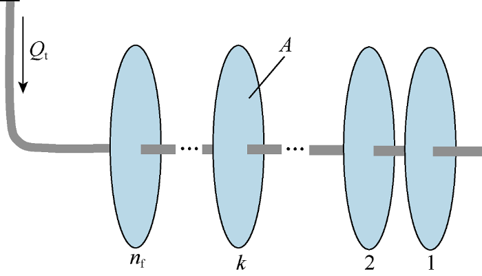
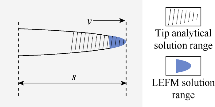
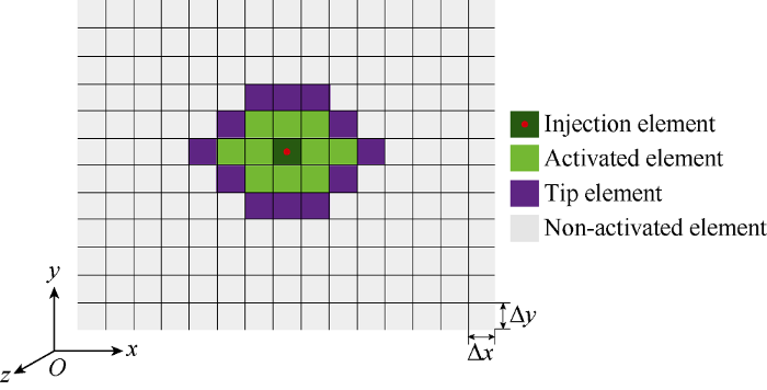
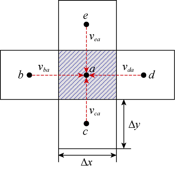

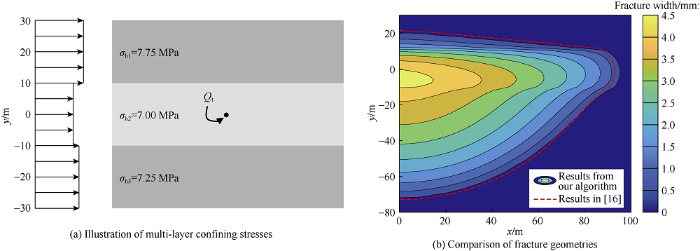
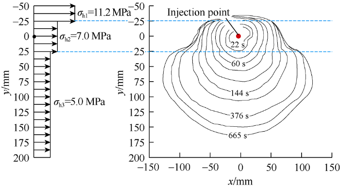
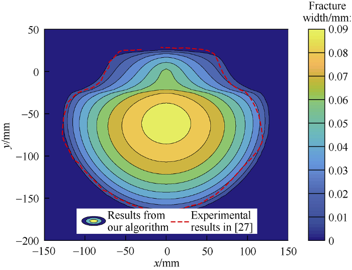
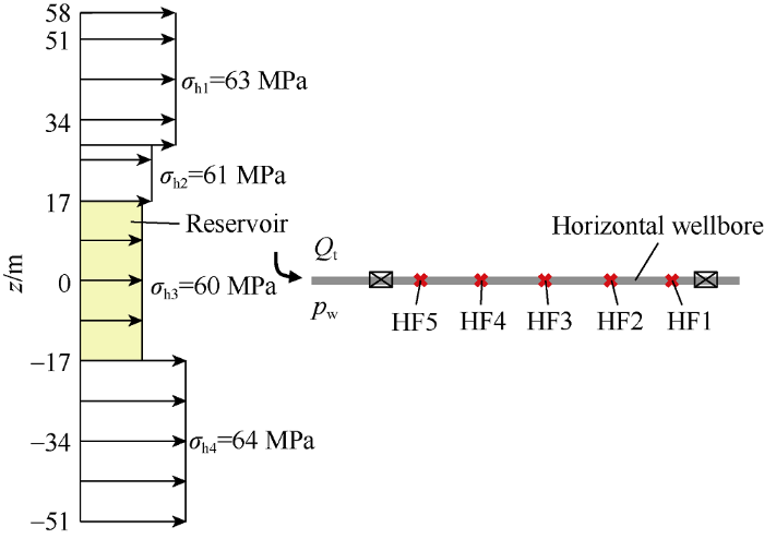
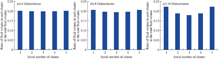
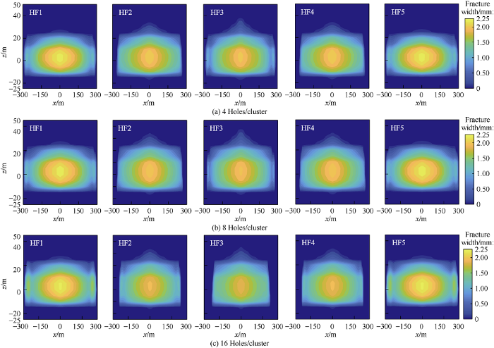
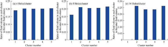
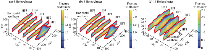
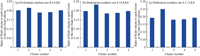
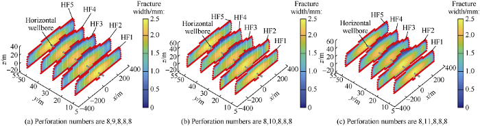
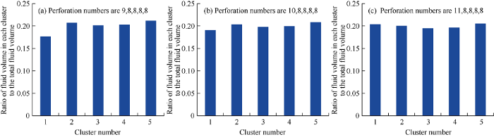
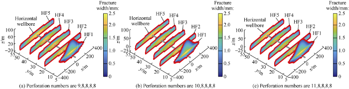
