Supported by the Scientific Research and Technological Development Project of CNPC. 2019A-3608
Abstract
A scaling-down experiment system of array laterolog resistivity was developed, and a corresponding formation model was built by 3D finite element numerical method to study the effect of different factors on the logging response quantitatively. The error between the experimental and numerical results was less than 5%, validating the reliability of the numerical simulation method. The single factor analysis of the formation relative dip, resistivity anisotropy and drilling fluid invasion was carried out by numerical simulation method, and the results show that: (1) The increase of relative dip can lead to the increase of formation resistivity, but the increasing value is relatively small, and the values of five array resistivity curves will reverse when the relative dip angle reaches a certain degree. (2) The increase of anisotropy coefficient λ can also cause the formation resistivity to rise, and the resistivity will increase by about 10% when λ increases from 1.0 to 1.5 in vertical wells. (3) Drilling fluid invasion has a more significant effect on the logging response than the former two factors. The order of the five curves will change due to drilling fluid invasion in anisotropic formation and the change rule is contrary to resistivity anisotropy. Taking the logging data of the Yingxi oilfield in the Qaidam Basin as an example, an anisotropic formation model considering drilling fluid invasion was built, and the numerical simulation results from the above methods were basically consistent with the logging data, which verified the accuracy of the method again. The results of this study lay a theoretical foundation for multiple-parameter inversion in anisotropic formation under complex well conditions.
YUAN Chao, LI Chaoliu, ZHOU Cancan, XIAO Qiyao, LI Xia, FAN Yiren, YU Jun, WANG Lei, XING Tao. Forward simulation of array laterolog resistivity in anisotropic formation and its application. [J], 2020, 47(1): 80-88 doi:10.1016/S1876-3804(20)60007-6
Introduction
The foreland high and steep structure zones in the central and western basins of China are the main areas of petroleum exploration at present[1]. The extremely complex responses of resistivity logging due to tectonic uplift, resistivity anisotropy and drilling fluid invasion lead to low coincidence rate of logging interpretation in these areas, which seriously hinders the exploration and reserves calculation. The key to the problem is that there existing differences between the apparent resistivity and horizontal resistivity[2,3,4]. Array laterolog can provide several resistivity logging curves with different depths of investigation, and can well characterize formation resistivity anisotropy[5,6]. Through inverse modeling, fairly authentic formation horizontal resistivity can be obtained from array laterolog. At present, Schlumberger's high resolution array lateralog instrument HRLA[7] is widely used in China, and many researchers have also carried out related studies on the array laterolog. Liu et al. calculated the array lateralog response based on finite element method with stable flow field[8]. Wu et al. investigated the effects of borehole, surrounding rocks and drilling fluid invasion, etc. on the array laterolog response by forward simulation[9]. Deng et al. simulated the array laterolog response in fractured reservoirs based on three- dimensional finite element method[10,11]. Feng et al. studied the response characteristics in thin inter-bedding and inclined wells of array laterolog instrument HAL of CNPC by numerical simulation[12]. Chen conducted inversion study of array lateral logging with Marquardt method[13]. However, the previous studies lack quantitative analysis of the effects of different environmental factors on the array laterolog response.
In this study, the array laterolog response was investigated based on three-dimensional finite element numerical simulation method. And then, anisotropic formation models were constructed in the laboratory, and physical simulation experiments were carried out by using the scale-down array laterolog instrument to validate the reliability of the numerical simulation method. Furthermore, the effects of formation relative dip, resistivity anisotropy and drilling fluid invasion on the array laterolog response were simulated and quantitatively analyzed by the numerical method, and the research results were applied to the analysis of field data.
1. 3D numerical simulation principle of array laterolog
1.1. Principle of array laterolog
Compared with dual laterolog, the array laterolog can measure several apparent resistivity logging curves at different depths of investigation with higher vertical resolution and more radial detecting information, which can provide abundant information of invasion zone and formation resistivity[14,15]. At present, the commonly used logging tools include HRLA[16] of Schlumberger Company and HDLL[17] of Atlas Company. This study mainly focuses on HRLA of Schlumberger Company.
The structure of the electrode system of HRLA instrument[18] is shown in Fig. 1, which is composed of the main electrode (A0), six pairs of electrodes (A1-A6) and two pairs of supervisory electrodes (M0 and M1b). Six resistivity curves at different depths of investigation can be measured by changing the different combinations of the emission current and receiving currents of the electrodes.
Fig. 1.
Structural schematic of electrode system of HRLA instrument.
1.2. 3D finite element FEM simulation method
According to the finite element theory, the forward calculation of array laterolog response can be transformed into the problem of finding the extremum of function shown in equation (1)[19,20].
There are two different kinds of boundary conditions in the forward calculation model: Dirichlet and Neumann boundary conditions. At infinite distant formation boundary, the potential satisfies the Dirichlet boundary condition, then:
By solving the above large linear sparse equations, the electric field generated by arbitrary emission electrodes in the formation can be obtained. To obtain HRLA logging curves of different modes, it is necessary to focus the currents generated by different emission electrodes.
2. Physical experiment of scale-down array laterolog instrument
2.1. Experimental tool and instrument
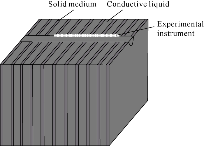
To verify the accuracy of three-dimensional finite element numerical simulation and find out the response law of array laterolog, a scale-down logging instrument was developed based on the array laterolog tool HRLA of Schlumberger company, and a water tank measuring model was designed to carry out experimental measurements. The conductive liquid and solid media were used as the surrounding rocks and target formation. A horizontal half-space measuring method was used to conduct the measurement (i.e. the instrument was placed horizontally, half in the conductive liquid and half in air), as shown in Fig. 2.
Fig. 2.
Schematic of the horizontal half-space measuring method.
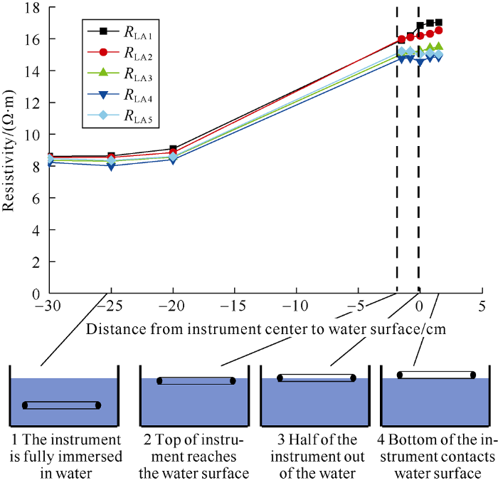
In order to find out the relationship between resistivity values measured by horizontal half-space measuring method (half-space for short) and full-space method (the instrument is all placed in the conductive liquid), the scale-down instrument was horizontally placed in the water tank filled with the conductive liquid, and 5 resistivity values RLA1-RLA5 at different positions were measured while the instrument was lifting, as shown in Fig. 3.
Fig. 3.
Diagrams of half-space and full-space measuring methods and the measurement results.
It can be seen from the experimental results that the resistivity measured by half-space method is about 1.86 times of that measured by full-space method. Therefore, the measurement results of half-space method can be converted to the real values of full-space resistivity measurement, but the half-space measuring method can minimize the area occupied by the experimental model and improve the material reuse rate, and it is also convenient for the measurement and maintenance of the experimental device.
2.2. Comparison of physical and numerical simulation results
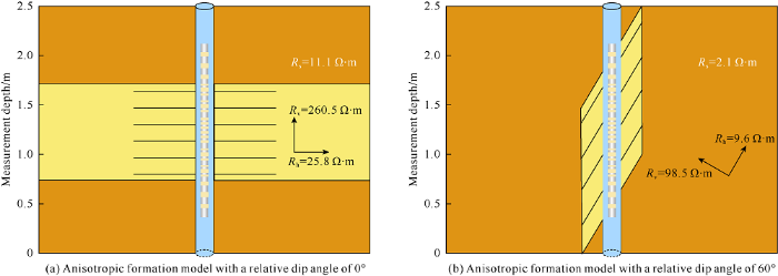
The anisotropic formation models with relative dip angles of 0° and 60° were made, and the diagrams of the two formation models are shown in Fig. 4a, 4b.
Fig. 4.
Diagram of anisotropic formation models and water tank used in the experiments.
The theoretical resistivity values of surrounding rocks and targeting formations in the experimental models were obtained through measuring the resistivity of the conductive liquid and the solid medium. In the formation model with a relative dip angle of 0° shown in Fig. 4a, the resistivity of surrounding rock is 11.1 Ω·m, and the horizontal and vertical resistivities of target formation are 25.8 Ω·m and 260.5 Ω·m respectively; in the model with relative dip angle of 60° shown in Fig. 4b, the resistivity of surrounding rock is 2.1 Ω·m, and the horizontal and vertical resistivities of target formation are 9.6 Ω·m and 98.5 Ω·m respectively.
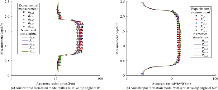
The resistivity responses in the formation models were measured with the scale-down instrument, and the logging response was also simulated by numerical simulation. The comparison between the experimental measurements and numerical simulation results is shown in Fig. 5.
Fig. 5.
Comparison of the results from experimental measurement and numerical simulation of formation models with the relative dip angle of 0o and 60o.
From Fig. 5, it can be seen that the results from experimental measurement are consistent with the results from numerical simulation. The error analysis between the results from experimental measurement and numerical simulation at the center point of the formation model is listed in Table 1, and the errors of most data points are lower than 5%, so the results of experimental measurement validate the reliability of the numerical simulation results.
Table 1
Table 1Error analysis between the results from experimental measurement and numerical simulation.
Different formation models were designed, and the effects of different factors, including formation relative dip, formation resistivity anisotropy and drilling fluid invasion, on the array laterolog response were simulated with the three-dimensional finite element method. In order to find out the variation range of anisotropy coefficient, the model parameters were set scientifically. The anisotropy coefficients of outcrop rocks of shale-sand interbed were measured in the laboratory. The outcrop rocks were cut into 3 cubic samples of 5 cm × 5 cm × 5 cm. The angle θ between rock bedding and horizontal direction of the 3 samples are respectively 0°, 30° and 80°, and the samples were coded as C1, C2 and C3 respectively, as shown in Fig. 6.
Fig. 6.
Pictures of cubic rock samples with different relative dip angles.
The vertical direction was specified as Z axis, and the X and Y-axis were specified by using the right-hand rule. The resistivity values of cubic rock samples in the directions of x, y and z axis (marked as Rx, Ry and Rz) were measured with electrode method. The resistivity parallel to and perpendicular to the bedding direction are respectively Rh and Rv. The rela-tionships between the resistivity values in the direction of x, y and z axis (Rx, Ry and Rz) and those parallel to and perpendicular to the bedding direction (Rh and Rv) can be expressed as follows:
The bedding of the rock samples is very developed, and the corresponding resistivity anisotropy of the samples are also very strong, which basically represent the maximum anisotropy coefficients in actual formations. From the measurement results, the maximum anisotropy coefficient is 2.43, so the anisotropy coefficient of the formation model was set at no more than 2.5.
3.1. Effect of formation relative dip
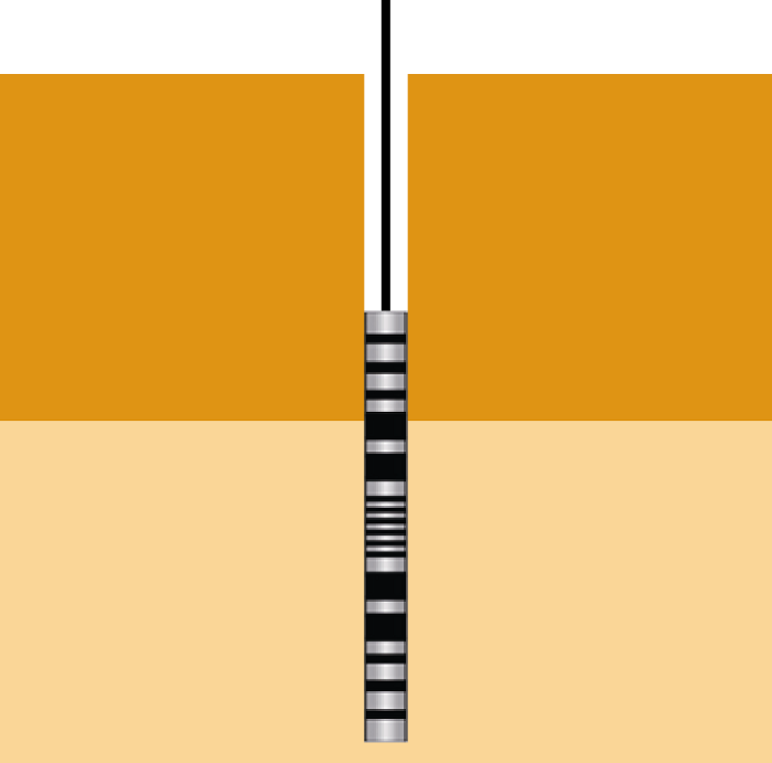
The two-layer formation model as shown in Fig. 7 was built, in which the borehole diameter was 20 cm; the resistivity of drilling fluid was 0.1 Ω·m. The light and dark yellow represent respectively low and high resistivity media; and the two layers in the model were set at the resistivity of 2 Ω·m and 4 Ω·m, 2 Ω·m and 20 Ω·m. The scale-down log instrument was used to measure the log responses when passing through the formation models at different formation relative dip angles. The response of deep resistivity curve (RLA5) of array laterolog is shown in Fig. 8.
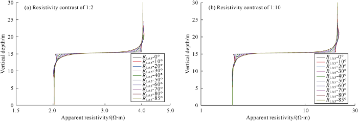
Fig. 8.
Simulated results of deep resistivity curve (RLA5) in two-layer formation models with different resistivity contrasts.
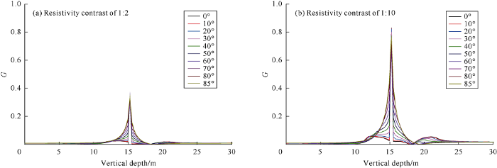
In order to study the effect of formation relative dip on the laterolog response quantitatively, the changing sensitivity of resistivity logging curve is defined as:
$G=\left| {{R}_{a}}-{{R}_{t}} \right|/{{R}_{t}}$
Fig. 9 shows the sensitivity of the logging instrument to resis-tivity change when passing through the two-layer formation model at different formation relative dip angles calculated by equation (7).
Fig. 9.
Changing sensitivity of array laterolog response in formation models with different resistivity contrasts.
It can be seen from Fig. 9 that the effect of formation relative dip angle on the array laterolog response is related to resistivity contrast. The bigger the resistivity contrast is, the larger the increase of apparent resistivity caused by the increase of formation relative dip angle at the formation interface is. At the formation resistivity contrasts of 1:2 and 1:10 when the relative dip angle of 40°, the relative variations of resistivity caused by the change of relative dip angle are 6% and 10%, respectively. Clearly, the formation relative dip has slight influence on the array laterolog response.
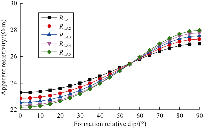
In order to study the response regularity of array laterolog resistivity in anisotropic formation with formation relative dip angle, an infinite formation model was built, and the model parameters were: borehole diameter of 20 cm, drilling fluid resistivity of 0.1 Ω·m, horizontal resistivity of 20 Ω·m, and anisotropy coefficient λ of 1.5. The relationship of the array laterolog resistivity and the formation relative dip was simulated and shown in Fig. 10.
Fig. 10.
Relationship between the array laterolog resistivity and the formation relative dip in anisotropic formation.
It can be seen from Fig. 10 that the increase of relative dip angle in anisotropic formation will lead to the increase of apparent resistivity. In the formation with an anisotropy coefficient of 1.5, the changes of the apparent deep resistivity (RLA5) and shallow resistivity (RLA1) caused by the relative dip angle change from 0° to 80° are 15% and 25% respectively. When the formation relative dip angle reaches 56.5°, the values of the five resistivity curves (RLA1-RLA5) reverse. At the reversing dip angle, the five resistivity curves have the same value, which is the blind point for identifying formation anisotropy in array laterolog inversion. When changing drilling fluid resistivity and formation horizontal resistivity, the dip angle of anisotropy causing the reverse of the five curve values would change somewhat. Through a large amount of numerical simulations, the reversing dip is from 40o to 65o.
3.2. Effect of formation resistivity anisotropy
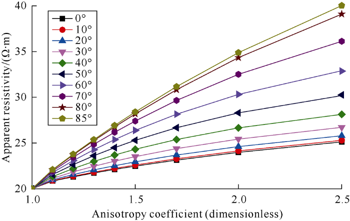
An infinite formation model was set up, with a borehole of 20 cm in diameter, drilling fluid resistivity of 0.1 Ω·m, and horizontal formation resistivity of 20 Ω·m. Under different formation relative dip angles, the formation anisotropy coefficient λ was changed from 1.0 to 2.5 to simulate the variation of deep resistivity RLA5 with formation anisotropy coefficient. The results are shown in Fig. 11.
Fig. 11.
Relationship between RLA5 and anisotropy coefficient at different formation relative dip angles.
It can be seen from the figure that at a constant formation relative dip angle, the larger the anisotropy coefficient is, the larger the apparent resistivity is. The increase of the formation resistivity anisotropy will lead to the increase of the apparent resistivity. When the formation relative dip angle is 0° and 85°, the increase of formation anisotropic coefficientλfrom 1.0 (isotropy) to 1.5 will cause apparent resistivity to increase by 1.1 times and 1.4 times. The larger the relative dip angle is, the more obvious the increase of apparent resistivity caused by the increase of the formation anisotropy coefficient will be.
3.3. Effect of drilling fluid invasion
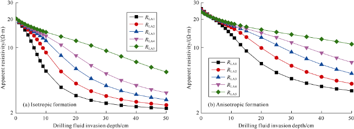
The parameters of formation model with drilling fluid invasion were: the borehole diameter of 20 cm, the drilling fluid resistivity of 0.1 Ω·m, the formation relative dip angle of 0°, horizontal resistivity of invaded zone and undisturbed formation of 2 Ω·m and 20 Ω·m respectively. The array laterolog responses in the isotropic and anisotropic formation (λ=2.0) with different drilling fluid invasion depths were simulated, and the results are shown in Fig. 12.
Fig. 12.
Array laterolog responses in isotropic and anisotropic formation with different drilling fluid invasion depths.
It can be seen from the Fig. 12 that the drilling fluid invasion has a more significant effect on array laterolog response than the formation relative dip and resistivity anisotropy. In the isotropic formation invaded by low-resistivity drilling fluid (Fig. 12a), when the drilling fluid invasion depth is 25 cm, the values of the deep resistivity (RLA5) and shallow resistivity (RLA1) decrease by 30% and 70% respectively. In the anisotropic formation invaded by low-resistivity drilling fluid (Fig. 12b), the five resistivity curves show negative and positive difference when the invasion depth is less than 12 cm and more than 12 cm respectively, so the drilling fluid invasion can change the order of five resistivity curves but its effect is opposite to resistivity anisotropy.
4. Analysis of field logging
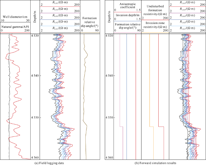
The Fig. 13a shows the well logging data of 4 530-4 560 m in Well S of Yingxi Oilfield in the Qaidam Basin. In this well section, the five laterolog resistivity curves show positive difference, and the formation relative dip angle is less than 30°. But according to the relationship curve of the array laterolog apparent resistivity and the formation relative dip angle shown in Fig. 10, the five laterolog resistivity curves should have negative difference when the formation relative dip is less than 30°, which means that the formation in this well section is invaded by low-resistivity drilling fluid. In addition, from the simulation results in Fig. 10 and Fig. 11, the value of RLA5/RLA1 is generally less than 2 when relative dip angle and formation resistivity anisotropy have effect on the array laterolog response, but the value of RLA5/RLA1 in this section is between 2 and 5, which suggests that the influence of drilling fluid invasion is greater than that of resistivity anisotropy. According to the analysis of logging data, the anisotropic formation model considering drilling fluid invasion was constructed, and the parameters of the formation model were:
(1) Borehole environment: According to the field data, water-based drilling fluid was used in this well, the drilling fluid resistivity was small and set at 0.1 Ω·m;
(2) Drilling fluid invasion depth: The RLA5/RLA1 value in this section of well is about 3.0, and the invasion depth was set at 0.7 m according to the array laterolog response in formations with different invasion depths shown in Fig. 12.
(3) Resistivity anisotropic coefficient: According to the core analysis data, the resistivity anisotropy coefficient of this section was about 1.2.
(4) Formation horizontal resistivity: From the resistivity log curve, this well section can be divided into two sub-sections: 4 530-4 552 m and 4 552-4 560 m, which need to set resistivity parameters separately. When the invasion depth is 0.7 m, the RLA1 curve is most affected by the resistivity in invaded zone, the horizontal resistivities of invaded zone in two sub-sections were respectively set at 8 Ω·m and 15 Ω·m considering the anisotropy coefficient of 1.2. According to the above known information and the deep resistivity curve RLA5, the horizontal resistivities of undisturbed formation in the two sub-sections were respectively set at 35 Ω·m and 85 Ω·m.
Fig. 13.
Comparison between the field logging data and the simulation results of Well S in Yingxi oilfield, the Qaidam Basin.
According to the above analysis of field logging data based on the forward simulation results, the anisotropy coefficient, drilling fluid invasion depth, formation relative dip, and the horizontal resistivity of the invasion zone and undisturbed formation horizontal resistivity in the formation model are shown in Fig. 13b. With these formation model parameters, the corresponding formation model was built to simulate the array laterolog resistivity response. The comparison between the field logging data and the simulation results is shown in Fig. 13b.
In Fig. 13b, it can be seen from the comparison analysis results that the simulated array laterolog curves by using the constructed anisotropic formation model considering drilling fluid invasion are basically consistent with the field logging data. The results also show that the array laterolog resistivity in this well is seriously affected by drilling fluid invasion, resulting in the low-resistivity invasion characteristics, whereas the formation relative dip and resistivity anisotropy are not the main factors affecting the resistivity. The field application results not only verify the accuracy of forward simulation and the rules of array laterolog responses, but also provide a theoretical basis for multi-parameter inversion of array laterolog resistivity in anisotropic formation under complex conditions considering formation resistivity anisotropy, formation relative dip and drilling fluid invasion.
5. Conclusions
The error between physical experiment results of the scale-down array laterolog resistivity and 3D finite element numerical simulation results is less than 5%, which verifies the reliability of numerical simulation. The effects of different factors on the array laterolog response were simulated and quantitatively analyzed by numerical simulation method. The results show that: the formation relative dip has slight effect on the logging response, and also controlled by the formation resistivity contrast; when the formation relative dip reaches a certain value in anisotropic formation, the values of the five laterolog resistivity curves will reverse; the formation resistivity anisotropy also can cause the increase of formation resistivity and is controlled by the formation relative dip; the drilling fluid invasion has a significant effect on the logging response and can change the order of the five resistivity curves of array laterolog, but the changing rule is opposite to that of formation resistivity anisotropy.
The research results were used to analyze the field logging data of Yingxi oilfield in the Qaidam Basin. The anisotropic formation model considering drilling fluid invasion was constructed, and the forward simulation results are basically consistent with the field logging data, which verifies the accuracy of the method again, and provides a theoretical basis for multi-parameter inversion of array laterolog resistivity in anisotropic formation under complex conditions.
Nomenclature
b—vector composed of current source applied at grid subdivision point;
en—normal unit vector, dimensionless;
E—electrode;
F(Φ)—functional equation;
G—changing sensitivity of resistivity logging curve, dimensionless
IE—current of the emission electrode, A;
js—current density on the surface of constant current electrode, A/m2;
K—stiffness matrix of finite element;
Ra—apparent resistivity of array laterolog, Ω·m;
Rh —resistivity parallel to the bedding direction, Ω·m;
RLA1, RLA2, RLA3, RLA4 and RLA5—five resistivity curves at different depths of investigation of array laterolog, Ω·m;
Rs—resistivity of surrounding rock, Ω·m;
Rt—true formation resistivity, Ω·m;
Rx—resistivity value in the direction of X, Ω·m;
Ry—resistivity value in the direction of Y, Ω·m;
Rz—resistivity value in the direction of Z, Ω·m;
Rv—resistivity perpendicular to the bedding direction, Ω·m;
UE—potential of the emission electrode, V;
V—calculation space excluding the electrode part, m3;
ΓI—boundary of insulation ring;
ΓC—boundary of emission and receiving electrodes;
α—formation relative dip angle, defined as the angle between the borehole and the normal direction of formation interface, (°);
θ—angle between rock bedding and horizontal direction, (°);
${{\xi }_{i}}$,${{\xi }_{j}}$—position on the x, y, or z axis in a rectangular coordinate system (When subscript i or j is 1, 2 and 3, it is the position on x, y and z axis respectively), m;
σ—conductivity, S/m;
${{\sigma }_{{{\xi }_{i}}{{\xi }_{j}}}}$—medium conductivity along the direction of ${{\xi }_{i}}{{\xi }_{j}}$, S/m;
Φ—potential at any point in the formation, V;
$\tilde{\Phi }$—vector composed of potential value to be calculated at grid subdivision point;
A fracture evaluation by acoustic logging technology in oil-based mud: A case from tight sandstone reservoirs in Keshen area of Kuqa Depression, Tarim Basin, NW China
Petroleum Exploration and Development, 2017,44(3):389-397.
A fracture evaluation by acoustic logging technology in oil-based mud: A case from tight sandstone reservoirs in Keshen area of Kuqa Depression, Tarim Basin, NW China
1
2017
... The foreland high and steep structure zones in the central and western basins of China are the main areas of petroleum exploration at present[1]. The extremely complex responses of resistivity logging due to tectonic uplift, resistivity anisotropy and drilling fluid invasion lead to low coincidence rate of logging interpretation in these areas, which seriously hinders the exploration and reserves calculation. The key to the problem is that there existing differences between the apparent resistivity and horizontal resistivity[2,3,4]. Array laterolog can provide several resistivity logging curves with different depths of investigation, and can well characterize formation resistivity anisotropy[5,6]. Through inverse modeling, fairly authentic formation horizontal resistivity can be obtained from array laterolog. At present, Schlumberger's high resolution array lateralog instrument HRLA[7] is widely used in China, and many researchers have also carried out related studies on the array laterolog. Liu et al. calculated the array lateralog response based on finite element method with stable flow field[8]. Wu et al. investigated the effects of borehole, surrounding rocks and drilling fluid invasion, etc. on the array laterolog response by forward simulation[9]. Deng et al. simulated the array laterolog response in fractured reservoirs based on three- dimensional finite element method[10,11]. Feng et al. studied the response characteristics in thin inter-bedding and inclined wells of array laterolog instrument HAL of CNPC by numerical simulation[12]. Chen conducted inversion study of array lateral logging with Marquardt method[13]. However, the previous studies lack quantitative analysis of the effects of different environmental factors on the array laterolog response. ...
Log evaluation of reservoir validity from formation stress in Kuche Foreland Basin
1
2018
... The foreland high and steep structure zones in the central and western basins of China are the main areas of petroleum exploration at present[1]. The extremely complex responses of resistivity logging due to tectonic uplift, resistivity anisotropy and drilling fluid invasion lead to low coincidence rate of logging interpretation in these areas, which seriously hinders the exploration and reserves calculation. The key to the problem is that there existing differences between the apparent resistivity and horizontal resistivity[2,3,4]. Array laterolog can provide several resistivity logging curves with different depths of investigation, and can well characterize formation resistivity anisotropy[5,6]. Through inverse modeling, fairly authentic formation horizontal resistivity can be obtained from array laterolog. At present, Schlumberger's high resolution array lateralog instrument HRLA[7] is widely used in China, and many researchers have also carried out related studies on the array laterolog. Liu et al. calculated the array lateralog response based on finite element method with stable flow field[8]. Wu et al. investigated the effects of borehole, surrounding rocks and drilling fluid invasion, etc. on the array laterolog response by forward simulation[9]. Deng et al. simulated the array laterolog response in fractured reservoirs based on three- dimensional finite element method[10,11]. Feng et al. studied the response characteristics in thin inter-bedding and inclined wells of array laterolog instrument HAL of CNPC by numerical simulation[12]. Chen conducted inversion study of array lateral logging with Marquardt method[13]. However, the previous studies lack quantitative analysis of the effects of different environmental factors on the array laterolog response. ...
The discovery and key exploration and prospecting technology of Yingdong oilfield in Qaidam Basin
1
2016
... The foreland high and steep structure zones in the central and western basins of China are the main areas of petroleum exploration at present[1]. The extremely complex responses of resistivity logging due to tectonic uplift, resistivity anisotropy and drilling fluid invasion lead to low coincidence rate of logging interpretation in these areas, which seriously hinders the exploration and reserves calculation. The key to the problem is that there existing differences between the apparent resistivity and horizontal resistivity[2,3,4]. Array laterolog can provide several resistivity logging curves with different depths of investigation, and can well characterize formation resistivity anisotropy[5,6]. Through inverse modeling, fairly authentic formation horizontal resistivity can be obtained from array laterolog. At present, Schlumberger's high resolution array lateralog instrument HRLA[7] is widely used in China, and many researchers have also carried out related studies on the array laterolog. Liu et al. calculated the array lateralog response based on finite element method with stable flow field[8]. Wu et al. investigated the effects of borehole, surrounding rocks and drilling fluid invasion, etc. on the array laterolog response by forward simulation[9]. Deng et al. simulated the array laterolog response in fractured reservoirs based on three- dimensional finite element method[10,11]. Feng et al. studied the response characteristics in thin inter-bedding and inclined wells of array laterolog instrument HAL of CNPC by numerical simulation[12]. Chen conducted inversion study of array lateral logging with Marquardt method[13]. However, the previous studies lack quantitative analysis of the effects of different environmental factors on the array laterolog response. ...
Explanation of earth stress logging and effectiveness evaluation of tight- sand reservoir in Dabei Area with steep structure
1
2014
... The foreland high and steep structure zones in the central and western basins of China are the main areas of petroleum exploration at present[1]. The extremely complex responses of resistivity logging due to tectonic uplift, resistivity anisotropy and drilling fluid invasion lead to low coincidence rate of logging interpretation in these areas, which seriously hinders the exploration and reserves calculation. The key to the problem is that there existing differences between the apparent resistivity and horizontal resistivity[2,3,4]. Array laterolog can provide several resistivity logging curves with different depths of investigation, and can well characterize formation resistivity anisotropy[5,6]. Through inverse modeling, fairly authentic formation horizontal resistivity can be obtained from array laterolog. At present, Schlumberger's high resolution array lateralog instrument HRLA[7] is widely used in China, and many researchers have also carried out related studies on the array laterolog. Liu et al. calculated the array lateralog response based on finite element method with stable flow field[8]. Wu et al. investigated the effects of borehole, surrounding rocks and drilling fluid invasion, etc. on the array laterolog response by forward simulation[9]. Deng et al. simulated the array laterolog response in fractured reservoirs based on three- dimensional finite element method[10,11]. Feng et al. studied the response characteristics in thin inter-bedding and inclined wells of array laterolog instrument HAL of CNPC by numerical simulation[12]. Chen conducted inversion study of array lateral logging with Marquardt method[13]. However, the previous studies lack quantitative analysis of the effects of different environmental factors on the array laterolog response. ...
Numerical simulation of mud invasion and its array laterolog response in deviated wells
1
2010
... The foreland high and steep structure zones in the central and western basins of China are the main areas of petroleum exploration at present[1]. The extremely complex responses of resistivity logging due to tectonic uplift, resistivity anisotropy and drilling fluid invasion lead to low coincidence rate of logging interpretation in these areas, which seriously hinders the exploration and reserves calculation. The key to the problem is that there existing differences between the apparent resistivity and horizontal resistivity[2,3,4]. Array laterolog can provide several resistivity logging curves with different depths of investigation, and can well characterize formation resistivity anisotropy[5,6]. Through inverse modeling, fairly authentic formation horizontal resistivity can be obtained from array laterolog. At present, Schlumberger's high resolution array lateralog instrument HRLA[7] is widely used in China, and many researchers have also carried out related studies on the array laterolog. Liu et al. calculated the array lateralog response based on finite element method with stable flow field[8]. Wu et al. investigated the effects of borehole, surrounding rocks and drilling fluid invasion, etc. on the array laterolog response by forward simulation[9]. Deng et al. simulated the array laterolog response in fractured reservoirs based on three- dimensional finite element method[10,11]. Feng et al. studied the response characteristics in thin inter-bedding and inclined wells of array laterolog instrument HAL of CNPC by numerical simulation[12]. Chen conducted inversion study of array lateral logging with Marquardt method[13]. However, the previous studies lack quantitative analysis of the effects of different environmental factors on the array laterolog response. ...
Fast modeling and practical inversion of laterolog-type downhole resistivity measurements
1
2018
... The foreland high and steep structure zones in the central and western basins of China are the main areas of petroleum exploration at present[1]. The extremely complex responses of resistivity logging due to tectonic uplift, resistivity anisotropy and drilling fluid invasion lead to low coincidence rate of logging interpretation in these areas, which seriously hinders the exploration and reserves calculation. The key to the problem is that there existing differences between the apparent resistivity and horizontal resistivity[2,3,4]. Array laterolog can provide several resistivity logging curves with different depths of investigation, and can well characterize formation resistivity anisotropy[5,6]. Through inverse modeling, fairly authentic formation horizontal resistivity can be obtained from array laterolog. At present, Schlumberger's high resolution array lateralog instrument HRLA[7] is widely used in China, and many researchers have also carried out related studies on the array laterolog. Liu et al. calculated the array lateralog response based on finite element method with stable flow field[8]. Wu et al. investigated the effects of borehole, surrounding rocks and drilling fluid invasion, etc. on the array laterolog response by forward simulation[9]. Deng et al. simulated the array laterolog response in fractured reservoirs based on three- dimensional finite element method[10,11]. Feng et al. studied the response characteristics in thin inter-bedding and inclined wells of array laterolog instrument HAL of CNPC by numerical simulation[12]. Chen conducted inversion study of array lateral logging with Marquardt method[13]. However, the previous studies lack quantitative analysis of the effects of different environmental factors on the array laterolog response. ...
Improved resistivity interpretation utilizing a new array laterolog tool and associated inversion processing
1
1998
... The foreland high and steep structure zones in the central and western basins of China are the main areas of petroleum exploration at present[1]. The extremely complex responses of resistivity logging due to tectonic uplift, resistivity anisotropy and drilling fluid invasion lead to low coincidence rate of logging interpretation in these areas, which seriously hinders the exploration and reserves calculation. The key to the problem is that there existing differences between the apparent resistivity and horizontal resistivity[2,3,4]. Array laterolog can provide several resistivity logging curves with different depths of investigation, and can well characterize formation resistivity anisotropy[5,6]. Through inverse modeling, fairly authentic formation horizontal resistivity can be obtained from array laterolog. At present, Schlumberger's high resolution array lateralog instrument HRLA[7] is widely used in China, and many researchers have also carried out related studies on the array laterolog. Liu et al. calculated the array lateralog response based on finite element method with stable flow field[8]. Wu et al. investigated the effects of borehole, surrounding rocks and drilling fluid invasion, etc. on the array laterolog response by forward simulation[9]. Deng et al. simulated the array laterolog response in fractured reservoirs based on three- dimensional finite element method[10,11]. Feng et al. studied the response characteristics in thin inter-bedding and inclined wells of array laterolog instrument HAL of CNPC by numerical simulation[12]. Chen conducted inversion study of array lateral logging with Marquardt method[13]. However, the previous studies lack quantitative analysis of the effects of different environmental factors on the array laterolog response. ...
Calculation and characteristics of array laterlog responses
1
2002
... The foreland high and steep structure zones in the central and western basins of China are the main areas of petroleum exploration at present[1]. The extremely complex responses of resistivity logging due to tectonic uplift, resistivity anisotropy and drilling fluid invasion lead to low coincidence rate of logging interpretation in these areas, which seriously hinders the exploration and reserves calculation. The key to the problem is that there existing differences between the apparent resistivity and horizontal resistivity[2,3,4]. Array laterolog can provide several resistivity logging curves with different depths of investigation, and can well characterize formation resistivity anisotropy[5,6]. Through inverse modeling, fairly authentic formation horizontal resistivity can be obtained from array laterolog. At present, Schlumberger's high resolution array lateralog instrument HRLA[7] is widely used in China, and many researchers have also carried out related studies on the array laterolog. Liu et al. calculated the array lateralog response based on finite element method with stable flow field[8]. Wu et al. investigated the effects of borehole, surrounding rocks and drilling fluid invasion, etc. on the array laterolog response by forward simulation[9]. Deng et al. simulated the array laterolog response in fractured reservoirs based on three- dimensional finite element method[10,11]. Feng et al. studied the response characteristics in thin inter-bedding and inclined wells of array laterolog instrument HAL of CNPC by numerical simulation[12]. Chen conducted inversion study of array lateral logging with Marquardt method[13]. However, the previous studies lack quantitative analysis of the effects of different environmental factors on the array laterolog response. ...
Forward response analysis of array lateral logging tool
1
2008
... The foreland high and steep structure zones in the central and western basins of China are the main areas of petroleum exploration at present[1]. The extremely complex responses of resistivity logging due to tectonic uplift, resistivity anisotropy and drilling fluid invasion lead to low coincidence rate of logging interpretation in these areas, which seriously hinders the exploration and reserves calculation. The key to the problem is that there existing differences between the apparent resistivity and horizontal resistivity[2,3,4]. Array laterolog can provide several resistivity logging curves with different depths of investigation, and can well characterize formation resistivity anisotropy[5,6]. Through inverse modeling, fairly authentic formation horizontal resistivity can be obtained from array laterolog. At present, Schlumberger's high resolution array lateralog instrument HRLA[7] is widely used in China, and many researchers have also carried out related studies on the array laterolog. Liu et al. calculated the array lateralog response based on finite element method with stable flow field[8]. Wu et al. investigated the effects of borehole, surrounding rocks and drilling fluid invasion, etc. on the array laterolog response by forward simulation[9]. Deng et al. simulated the array laterolog response in fractured reservoirs based on three- dimensional finite element method[10,11]. Feng et al. studied the response characteristics in thin inter-bedding and inclined wells of array laterolog instrument HAL of CNPC by numerical simulation[12]. Chen conducted inversion study of array lateral logging with Marquardt method[13]. However, the previous studies lack quantitative analysis of the effects of different environmental factors on the array laterolog response. ...
Simulation of array laterolog response of fracture in fractured reservoir
1
2009
... The foreland high and steep structure zones in the central and western basins of China are the main areas of petroleum exploration at present[1]. The extremely complex responses of resistivity logging due to tectonic uplift, resistivity anisotropy and drilling fluid invasion lead to low coincidence rate of logging interpretation in these areas, which seriously hinders the exploration and reserves calculation. The key to the problem is that there existing differences between the apparent resistivity and horizontal resistivity[2,3,4]. Array laterolog can provide several resistivity logging curves with different depths of investigation, and can well characterize formation resistivity anisotropy[5,6]. Through inverse modeling, fairly authentic formation horizontal resistivity can be obtained from array laterolog. At present, Schlumberger's high resolution array lateralog instrument HRLA[7] is widely used in China, and many researchers have also carried out related studies on the array laterolog. Liu et al. calculated the array lateralog response based on finite element method with stable flow field[8]. Wu et al. investigated the effects of borehole, surrounding rocks and drilling fluid invasion, etc. on the array laterolog response by forward simulation[9]. Deng et al. simulated the array laterolog response in fractured reservoirs based on three- dimensional finite element method[10,11]. Feng et al. studied the response characteristics in thin inter-bedding and inclined wells of array laterolog instrument HAL of CNPC by numerical simulation[12]. Chen conducted inversion study of array lateral logging with Marquardt method[13]. However, the previous studies lack quantitative analysis of the effects of different environmental factors on the array laterolog response. ...
The simulation and analysis of array lateral log response of fracture in coalbed methane reservoir
1
2010
... The foreland high and steep structure zones in the central and western basins of China are the main areas of petroleum exploration at present[1]. The extremely complex responses of resistivity logging due to tectonic uplift, resistivity anisotropy and drilling fluid invasion lead to low coincidence rate of logging interpretation in these areas, which seriously hinders the exploration and reserves calculation. The key to the problem is that there existing differences between the apparent resistivity and horizontal resistivity[2,3,4]. Array laterolog can provide several resistivity logging curves with different depths of investigation, and can well characterize formation resistivity anisotropy[5,6]. Through inverse modeling, fairly authentic formation horizontal resistivity can be obtained from array laterolog. At present, Schlumberger's high resolution array lateralog instrument HRLA[7] is widely used in China, and many researchers have also carried out related studies on the array laterolog. Liu et al. calculated the array lateralog response based on finite element method with stable flow field[8]. Wu et al. investigated the effects of borehole, surrounding rocks and drilling fluid invasion, etc. on the array laterolog response by forward simulation[9]. Deng et al. simulated the array laterolog response in fractured reservoirs based on three- dimensional finite element method[10,11]. Feng et al. studied the response characteristics in thin inter-bedding and inclined wells of array laterolog instrument HAL of CNPC by numerical simulation[12]. Chen conducted inversion study of array lateral logging with Marquardt method[13]. However, the previous studies lack quantitative analysis of the effects of different environmental factors on the array laterolog response. ...
On response characteristics analysis of HAL tool in thin inter-beds and deviated hole formation
1
2013
... The foreland high and steep structure zones in the central and western basins of China are the main areas of petroleum exploration at present[1]. The extremely complex responses of resistivity logging due to tectonic uplift, resistivity anisotropy and drilling fluid invasion lead to low coincidence rate of logging interpretation in these areas, which seriously hinders the exploration and reserves calculation. The key to the problem is that there existing differences between the apparent resistivity and horizontal resistivity[2,3,4]. Array laterolog can provide several resistivity logging curves with different depths of investigation, and can well characterize formation resistivity anisotropy[5,6]. Through inverse modeling, fairly authentic formation horizontal resistivity can be obtained from array laterolog. At present, Schlumberger's high resolution array lateralog instrument HRLA[7] is widely used in China, and many researchers have also carried out related studies on the array laterolog. Liu et al. calculated the array lateralog response based on finite element method with stable flow field[8]. Wu et al. investigated the effects of borehole, surrounding rocks and drilling fluid invasion, etc. on the array laterolog response by forward simulation[9]. Deng et al. simulated the array laterolog response in fractured reservoirs based on three- dimensional finite element method[10,11]. Feng et al. studied the response characteristics in thin inter-bedding and inclined wells of array laterolog instrument HAL of CNPC by numerical simulation[12]. Chen conducted inversion study of array lateral logging with Marquardt method[13]. However, the previous studies lack quantitative analysis of the effects of different environmental factors on the array laterolog response. ...
Inversion method and application of array laterolog
1
2009
... The foreland high and steep structure zones in the central and western basins of China are the main areas of petroleum exploration at present[1]. The extremely complex responses of resistivity logging due to tectonic uplift, resistivity anisotropy and drilling fluid invasion lead to low coincidence rate of logging interpretation in these areas, which seriously hinders the exploration and reserves calculation. The key to the problem is that there existing differences between the apparent resistivity and horizontal resistivity[2,3,4]. Array laterolog can provide several resistivity logging curves with different depths of investigation, and can well characterize formation resistivity anisotropy[5,6]. Through inverse modeling, fairly authentic formation horizontal resistivity can be obtained from array laterolog. At present, Schlumberger's high resolution array lateralog instrument HRLA[7] is widely used in China, and many researchers have also carried out related studies on the array laterolog. Liu et al. calculated the array lateralog response based on finite element method with stable flow field[8]. Wu et al. investigated the effects of borehole, surrounding rocks and drilling fluid invasion, etc. on the array laterolog response by forward simulation[9]. Deng et al. simulated the array laterolog response in fractured reservoirs based on three- dimensional finite element method[10,11]. Feng et al. studied the response characteristics in thin inter-bedding and inclined wells of array laterolog instrument HAL of CNPC by numerical simulation[12]. Chen conducted inversion study of array lateral logging with Marquardt method[13]. However, the previous studies lack quantitative analysis of the effects of different environmental factors on the array laterolog response. ...
Numerical simulation of high resolution array lateral logging responses
1
2009
... Compared with dual laterolog, the array laterolog can measure several apparent resistivity logging curves at different depths of investigation with higher vertical resolution and more radial detecting information, which can provide abundant information of invasion zone and formation resistivity[14,15]. At present, the commonly used logging tools include HRLA[16] of Schlumberger Company and HDLL[17] of Atlas Company. This study mainly focuses on HRLA of Schlumberger Company. ...
Mathematical model and fast finite element modeling of high resolution array lateral logging
1
2013
... Compared with dual laterolog, the array laterolog can measure several apparent resistivity logging curves at different depths of investigation with higher vertical resolution and more radial detecting information, which can provide abundant information of invasion zone and formation resistivity[14,15]. At present, the commonly used logging tools include HRLA[16] of Schlumberger Company and HDLL[17] of Atlas Company. This study mainly focuses on HRLA of Schlumberger Company. ...
Better saturation from new array laterolog
1
1999
... Compared with dual laterolog, the array laterolog can measure several apparent resistivity logging curves at different depths of investigation with higher vertical resolution and more radial detecting information, which can provide abundant information of invasion zone and formation resistivity[14,15]. At present, the commonly used logging tools include HRLA[16] of Schlumberger Company and HDLL[17] of Atlas Company. This study mainly focuses on HRLA of Schlumberger Company. ...
Field measurements and inversion results of the high-definition lateral log
1
1998
... Compared with dual laterolog, the array laterolog can measure several apparent resistivity logging curves at different depths of investigation with higher vertical resolution and more radial detecting information, which can provide abundant information of invasion zone and formation resistivity[14,15]. At present, the commonly used logging tools include HRLA[16] of Schlumberger Company and HDLL[17] of Atlas Company. This study mainly focuses on HRLA of Schlumberger Company. ...
Forward simulation of array laterolog response
1
2009
... The structure of the electrode system of HRLA instrument[18] is shown in Fig. 1, which is composed of the main electrode (A0), six pairs of electrodes (A1-A6) and two pairs of supervisory electrodes (M0 and M1b). Six resistivity curves at different depths of investigation can be measured by changing the different combinations of the emission current and receiving currents of the electrodes. ...
Dual laterolog response in 3-D environments
1
2000
... According to the finite element theory, the forward calculation of array laterolog response can be transformed into the problem of finding the extremum of function shown in equation (1)[19,20]. ...
Numerical simulation and characteristics analysis of dual laterolog in cavernous reservoirs on the basis of 3D-FEM
1
2017
... According to the finite element theory, the forward calculation of array laterolog response can be transformed into the problem of finding the extremum of function shown in equation (1)[19,20]. ...
The role of electrical anisotropy in magnetotelluric response: From modelling and dimensionality analysis to inversion and interpretation
1
2014
... The definition of anisotropy coefficient λ is defined as[21]: ...


