Supported by the China National Science and Technology Major Project. 2017ZX05013-001 CNPC Science and Technology Major Research Project. 2018B-4907
Abstract
To evaluate the fracturing effect and dynamic change process after volume fracturing with vertical wells in low permeability oil reservoirs, an oil-water two-phase flow model and a well model are built. On this basis, an evaluation method of fracturing effect based on production data and fracturing fluid backflow data is established, and the method is used to analyze some field cases. The vicinity area of main fracture after fracturing is divided into different stimulated regions. The permeability and area of different regions are used to characterize the stimulation strength and scale of the fracture network. The conductivity of stimulated region is defined as the product of the permeability and area of the stimulated region. Through parameter sensitivity analysis, it is found that half-length of the fracture and the permeability of the core area mainly affect the flow law near the well, that is, the early stage of production; while matrix permeability mainly affects the flow law at the far end of the fracture. Taking a typical old well in Changqing Oilfield as an example, the fracturing effect and its changes after two rounds of volume fracturing in this well are evaluated. It is found that with the increase of production time after the first volume fracturing, the permeability and conductivity of stimulated area gradually decreased, and the fracturing effect gradually decreased until disappeared; after the second volume fracturing, the permeability and conductivity of stimulated area increased significantly again.
Keywords:volume fracturing
;
fracturing effect evaluation
;
fracturing area
;
conductivity
;
low permeability reservoir
;
vertical well
ZHANG Anshun, YANG Zhengming, LI Xiaoshan, XIA Debin, ZHANG Yapu, LUO Yutian, HE Ying, CHEN Ting, ZHAO Xinli. An evaluation method of volume fracturing effects for vertical wells in low permeability reservoirs. [J], 2020, 47(2): 441-448 doi:10.1016/S1876-3804(20)60061-1
Introduction
In recent years, low-permeability oil and gas reservoirs have gradually become the major targets of domestic oil and gas exploration and development, and oil reserves in low-permeability reservoirs have accounted for more than 70% of proven oil reserves[1]. Due to the small throat[2,3,4], low-permeability reservoirs are difficult to get energy replenished, so oil wells in them gradually decline in production, and become low-production and low-efficiency wells. China National Petroleum Corporation (hereinafter referred to as PetroChina) has more than 80 000 such low-production and low-efficiency vertical wells, and it is difficult to achieve the purpose of increasing production of them by conventional fracturing. In recent years, learning from the idea of volume fracturing in shale gas reservoirs, PetroChina has conducted volume re-fracturing tests in old wells (vertical wells) in Changqing, Jilin, Daqing and other oilfields, and achieved good results.
There are currently two main methods for evaluating the effect of volume fracturing. One is the direct method, which uses some fracture monitoring techniques such as microseismics, inclinometers, and distributed fiber optics to evaluate the stimulated reservoir volume after volume fracturing. Some researchers have used microseismic monitoring results to correct geological models after volume fracturing and predict development indexes for different fracturing schemes[5,6]. Some researchers have done a lot of research on stimulated reservoir volumes based on microseismic data and imaging results[7,8,9]. Some researchers have districted complex fracture networks based on fracture monitoring technologies such as microseismics, and performed sensitivity analysis and productivity prediction by given permeability of different districts[10,11,12]. The inclinometer simulates inversely formation parameters by measuring the amount of formation tilt caused by fractures, and then describes the complexity of fractures after volume fracturing[13,14]. Distributed optical fibers monitor fractures by measuring the contribution of fluid production profiles and the yield of each layer[15,16,17]. These direct methods can only evaluate the fracturing effect at a certain point after volume fracturing. The other is the indirect method, which uses mathematical methods to evaluate the effect of volume fracturing. Some researchers[5, 18-21] mainly considered the change of the number of fractures or skin factors in the near-well zone after volume fracturing, and evaluated the volume fracturing effect by simulating the production changes after volume fracturing. However, these studies did not address key issues such as the scope of the fracturing area and the half-length of the main fracture after volume fracturing. Xu et al.[22,23,24,25] and Meyer et al.[26,27] proposed the hydraulic fracture network model and discrete fracture network model respectively based on the material balance and momentum conservation equations in view of the characteristics of complex fracture network structures with high conductivity after volume fracturing in oil wells. However, these two models need to combine with fracturing construction parameters and in-situ stress parameters when calculating fracture and fracture network parameters, and cannot give the variation law of seepage field in the oil well during the production stage after fracturing. The product of fracture permeability and fracture width is commonly used to represent fracture conductivity[28,29], but there are many shortcomings in using this method to characterize the conductivity of the vertical well after fracturing. In this study, a numerical method is established that can evaluate the volume fracturing. A method characterizing the conductivity of stimulated reservoir area is proposed and applied to the field.
1. Numerical simulation model of volume fracturing
The hybrid grid was used to divide the reservoir (Fig. 1), and different types of grids were used according to fluid flow characteristics and complex geological characteristics of the reservoir after volume fracturing. A radial grid was used near the wellbore, and unstructured grid (perpendicular bisection) was used for the zone far away from the wellbore. This can not only reflect the fluid flow characteristics near the wellbore, but also accurately describe the fracture morphology of the formation after fracturing. At the same time, a higher simulation accuracy can be obtained with a smaller number of grids[30].
Fig. 1.
Schematic diagram of volume fracturing model and grid division in an oil reservoir.
1.1. Fluid seepage model
The fluid flow in the reservoir is governed by the oil-water two-phase seepage law. The numerical analysis in this study is based on the finite volume method. For the oil phase, there is the following equation:
The liquid production of oil wells will change during actual production. In the time period when the liquid production is constant, the time period is regarded as constant liquid production, and the production history is divided according to the time period.
For multilayer-fractured vertical wells, for the mth production layer, the bottom-hole inflow rate can be expressed as:
Similarly, the water production of the mth layer can be obtained.
The above are the oil-water two-phase flow model and well model. By linearizing the formulas (2), (3), (4), and (7) and combining the boundary conditions, the corresponding pressure field distribution and bottom hole pressure can be calculated. By fitting the calculated value of bottom hole pressure with the measured value, relevant fitting parameters can be obtained, and then the fracturing effect can be evaluated.
2. Evaluation method of volume fracturing effect
Based on the numerical simulation model of volume fracturing, to work out a numerical method evaluating volume fracturing effects, it is necessary to solve the problem of multiplicity of parameters in numerical methods. This requires the division of stimulated reservoir zones in vertical wells, parameter sensitivity analysis, and characterization of volume fracturing conductivity.
2.1. Validation of the numerical simulation model
In order to verify the correctness of the numerical simulation model, a geological model with an injection well and a production well was established (Fig. 2), this geological simulation model was used to calculate the pressure curve, and the pressure curve was compared with the simulation results of Eclipse software. The model was 200 m × 200 m on the plane, and the size of a single grid was 4 m × 4 m. The basic parameters of the model are shown in Table 1. The situation of constant liquid production at the daily rate of 10 m3 for 30 days was simulated. As can be seen from Fig. 3, the calculation results of the numerical simulation model established in this paper are consistent with the results from the Eclipse software, proving the model is reliable.
2.2. Division of volume fracturing area and characterization of conductivity in vertical wells
A volume fracturing vertical well in a rectangular closed boundary reservoir is taken as an example to illustrate the division of different volume fracturing zones (Fig. 4). The main stimulated zone of volume fracturing is the main fracturing zone or the core zone. This area has a high stimulated strength, so the fractures in this zone have high permeability and conductivity. The area affected by volume fracturing is the secondary fracture zone or external stimulated zone. Compared with the core zone, the fractures in this zone have lower permeability and conductivity. Outside of the affected zone is un-stimulated zone. Dividing the volume fracturing zones can effectively solve the problem of multiplicity of permeability and stimulated reservoir area during numerical simulation.
Fig. 4.
Schematic diagram of volume fracturing of vertical wells in a closed boundary reservoir.
In this paper, the newly-defined stimulated reservoir conductivity is used to describe the volume fracturing effect. The permeability and area of the fracturing area are used to characterize the strength and scale of the fracture network after fracturing. In fracturing area, the stimulated reservoir conductivity (SRC) is defined as the product of the permeability and area of the fracturing area. Due to the heterogeneous permeability in the fracturing area, the conductivity of the area is calculated using the following formula:
$SRC=\sum\limits_{k=1}^{M}{{{K}_{k}}{{A}_{k}}}$
2.3. Parameter sensitivity analysis
In this study, the fracturing effect was evaluated by using production data and fracturing fluid flowback data. Then, by analyzing the effects of various parameters on the fracturing curve after volume fracturing, the volume fracturing parameters and reservoir parameters were inversely obtained. In order to eliminate the multiple solutions of influencing factors, a parameter sensitivity analysis was performed.
It is assumed that there is a vertical well undergoing volume fracturing in the reservoir, and the size of the volume fracturing area is constant. We studied the effects of fracture half- length, core area permeability, and matrix permeability on bottom hole pressure. The basic parameters are shown in Table 2.
Table 2
Table 2Basic parameters of the volume fracturing vertical well in closed boundaries.
Fig. 5 shows the bottom hole pressure curves at different fracture half lengths. During calculation, the core zone permeability was 15×10-3 μm2, and the matrix permeability was 0.5×10⁻³ μm2. It can be seen from Fig. 5 that the fracture half- length mainly affects the early stage of the bottom hole pressure curve, and in the later stage, the bottom-hole pressure curves at different fracture half-lengths are almost parallel. Therefore, when the bottom hole pressure curve cannot be fitted at the early stage, the fracture half-length must be adjusted.
Fig. 5.
Curves of bottom hole pressure at different fracture half-lengths.
Fig. 6 shows the bottom hole flow pressure curves at different core zone permeabilities. During calculation, the half- length of the fracture was 120 m, and the matrix permeability was 0.5×10⁻³ μm2. It can be seen from Fig. 6 that in the early stage, bottom hole pressure curves at different core zone permeabilities are almost coincident, indicating that at this stage, compared with the half length of the fracture, the core zone permeability has little effect on the bottom hole pressure curve. At the later stage, the bottom hole pressure curves at different core zone permeabilities are almost parallel, indicating that the core zone permeability at this stage do not affect the fluid flow. Combining Fig. 5 and Fig. 6, it can be found that the fracture half-length and core zone permeability mainly affect the fluid flow near the wellbore, that is, the fluid flow regularity in the early production period, and the effect of fracture half-length is greater.
Fig. 6.
Curves of bottom hole pressure at different core zone permeabilities.
Fig. 7 shows the bottom hole pressure curves at different matrix permeabilities. In the calculation, the half-length of fracture was 120 m, and the core zone permeability was 15×10-3 μm2. It can be seen from Fig. 7 that matrix permeability affects the shape of bottom hole pressure curve. Matrix permeability mainly affects the fluid flow at the far end of the fracture. The lower the matrix permeability, the weaker the fluid flow capacity of the fracture distal end, which means that the smaller fluid flow capacity from matrix to fracture. In general, if the stress sensitivity isn’t considered, the matrix permeability is determined from the geological data available and is not adjusted.
Fig. 7.
Curves of bottom hole pressure at different matrix permeabilities.
3. Oilfield applications
3.1. Overview of the example well geology and development
A typical old well (Y well) in the Changqing Oilfield of the Ordos Basin was selected. The well is a vertical well targeting the Chang 62 and Chang 63 formation with relatively continuous distribution. The reservoirs 24 m thick in total, have a porosity of 12%, a permeability range of (0.2-0.3)×10-3 μm2, and an oil saturation of 56%. Due to the extremely low reservoir permeability, the well was fractured and put into production in 2007. In the early stage, it had a fairly high production, but the production declined rapidly, and soon the well became a low production well. Drawing on the concept of shale gas volume fracturing, the well was treated by volume fracturing in 2016 and 2018, respectively.
3.2. Evaluation of volume fracturing effect
In this paper, the production data of Well Y from the first volume fracturing in 2016 to the second volume fracturing in 2018 was used to evaluate the effect of the first volume fracturing of this well in 2016. For the second volume fracturing in 2018, due to the short production time, the fracturing fluid flowback data was used to evaluate the volume fracturing effect.
By processing the production data after the first volume fracturing, the curve of the bottom hole pressure over time was obtained by fitting. According to the fitting results, the production process of this well is divided into three stages, as shown in Fig. 8.
Fig. 8.
Fitting results of production curve of Well Y.
The first stage is from June 22, 2016 to September 19, 2016. For this stage, from calculation the core zone has a permeability of 15×10-3 μm2, fracturing area of 3 687.5 m2, and conductivity of 55 312.5×10⁻³ μm2·m2; the secondary fracture zone had a permeability of 1.5×10⁻³ μm2, an area of 13 382.52 m2, and a conductivity of 20 073.78×10⁻³ μm2·m2. Then the conductivity of fractured area in this stage was 75 386.28×10⁻³ μm2·m2. It can be seen from Fig. 9, as the production time increases, the pressures in the core zone and secondary fracture zone decrease sharply. At the 38th day into production, the pressure in the core zone dropped to 46.96% of the initial pressure, while the pressure in secondary fracture zone dropped to 61.19% of the initial pressure. The pressure drop in the core zone is larger than that in secondary fracture zone. At the 110th day into production, the pressure showed an overall drop trend, but the external energy supplementation effect was not obvious. Since the water cut of the first stage changed significantly, an oil-water two-phase model was used to fit the water cut of this stage. The fitting results are shown in Fig. 10. Combining with the fitting results of water saturation distribution at this stage, it can be concluded that the water saturation around the fractures was high after the fracturing.
Fig. 10.
Fitting results of water cut in the first stage.
The second stage is from November 26, 2016 to June 24, 2017. At this stage, from calculation, the core zone had a permeability of 8×10⁻³ μm2, an area of 3 687.5 m2, and a conductivity of 29 500×10-3 μm2·m2; the secondary fracture zone had a permeability of 1×10⁻³ μm2, an area of 12 904.06 m2, and a conductivity of 12 904.06×10⁻³ μm2·m2. Then the conductivity of stimulated area in this stage was 42 404.06× 10⁻³ μm2·m2. Compared with the first stage, the permeability and conductivity of in stimulated reservoir area in the second stage decreased both by nearly 50%. It can be seen from Fig. 11, the reservoir pressure in the second stage was relatively stable, and the external energy supplementation effect was obvious. The fitted reservoir boundary was a constant pressure boundary. At this stage, the bottom hole pressure was relatively stable, and in the later period, the bottom hole pressure increased slightly, which also indicates that there was some energy supplement at the boundary. This coincides with the fact that there is a water injection well near the well.
Fig. 11.
Formation pressure distribution in the second stage.
The third stage is from October 11, 2017 to May 6, 2018. At this stage, from calculate the core zone had a permeability of 0.8×10⁻³ μm2, fracturing area of 3 687.50 m2, and conductivity of 2 950×10-3 μm2·m2; the secondary fracture zone had a permeability of 0.5×10⁻³ μm2, area of 4 832.19 m2, and conductivity of 2 416.1×10⁻³ μm2·m2. Then the conductivity of the stimulated area in this stage was 5 493.48×10⁻³ μm2·m2. At this stage, the permeability and conductivity of the core zone decreased to 1/10 of those in the second stage respectively. The permeabilities of core zone and secondary fracture zone didn’t differ much from the matrix permeability, which indicates that the volume fracturing has gradually lost effect. At this stage, the bottom hole pressure was relatively stable, indicating that there was some energy supplement at the boundary, but the energy supplement effect was weak.
As the first volume fracturing lost effect, Well Y was re-fractured the second time in August 2018. Due to the short production time, fracturing fluid flowback data was used to evaluate the fracturing effect of this time. The flowback pressure curve is shown in Fig. 12. Because of the short fracturing fluid flowback time, the relevant data can only reflect the volume fracturing effect in the core zone. From calculation, the core zone had a permeability of 90×10-3 μm2, an area of 7241.89 m2, and a conductivity of 651 770.1×10⁻³ μm2·m2. Compared with the first stage of the first volume fracturing, the core zone increased by 5 times in permeability, nearly 1 time in area, and more than 10 times in conductivity.
Fig. 12.
Pressure over time during fracturing fluid flowback.
By analyzing the dynamic change process of the conductivity of the volume fracturing area, it can be found that with the elapse of time, the fracturing effect gradually decreases and disappears.
4. Conclusions
A numerical simulation model of volume fracturing for vertical wells in low-permeability reservoirs was established, and the problem of parameter multiplicity in numerical calculations was solved through volume fracturing area division, parameter sensitivity analysis, and volume fracturing conductivity characterization. Then a new method for evaluating the volume fracturing effect in vertical wells in low-permeability reservoirs has been formed. The volume fracturing area is divided into the core zone and secondary fracture zone. The conductivity of the stimulated area is defined as the product of its permeability and area. The conductivities of the core zone and secondary fracture zone were calculated separately, and the sum of them is the conductivity of the volume fracturing area. The parameter sensitivity analysis results show that the fracture half-length and core zone permeability mainly affect the fluid flow near the wellbore, that is, the fluid flow regularity in the early stage of production, and the effect of fracture half-length is greater. The matrix permeability mainly affects the fluid flow at the far end of the fracture.
The established method can evaluate the volume fracturing effect in different production stages after volume fracturing and reflect dynamic changes of fracturing effect over time. Application of the method in an actual oilfield well shows that the fracturing effect gradually decreases with the elapse of production time and disappears at last.
Nomenclature
Ak—Kth area, m2;
Bo, Bw—oil, water volume factor, m3/m3;
C—wellbore storage factor, m3/Pa;
dij—distance between center points of grid i and grid j, m;
dΩ—volume element, m3;
h—reservoir thickness, m;
i—grid number;
j—the number of grids adjacent to grid i;
Jo, Jw—oil and water production index, m3/(Pa·s);
k—zone number;
K—absolute permeability, m2;
Ki—absolute permeability of grid i, m2;
Kk—permeability of the Kth zone, 10-3 μm2;
Kro, Krw—relative permeability of oil and water, f;
m—production layer number;
M—number of zones;
n—time step number;
N—total production layers;
pcow—capillary pressure, Pa;
po—oil phase pressure, Pa;
pwf—bottom hole pressure, Pa;
px,m—pressure of grid x in the mth layer, Pa;
qb—well inflow, m3/s;
qb,m—liquid production of layer m, m3/s;
qo,m—oil production of layer m, m3/s;
qosc, qwsc—source items of oil and water under standard conditions, m3/s;
Qp—total production, m3/s;
Qs—production due to wellbore storage effect, m3/s;
rw—wellbore radius, m;
ro—reservoir radius, m;
S—skin factor, f;
So, Sw—oil and water saturation, f;
SRC—conductivity of stimulated reservoir, 10-3 μm2·m2;
Tij,o, Tij,w—conductivity of oil and water phases, m3/(Pa·s);
Vi—volume of grid i, m3;
x—number of the grid where the well in the m-th layer is located;
Z—depth, m;
β—liquid proportion of layer m in total liquid production;
Types, characteristics, genesis and prospects of conventional and unconventional hydrocarbon accumulations: Taking tight oil and tight gas in China as an instance
Study on pore structures of tight sandstone reservoirs based on nitrogen adsorption, high-pressure mercury intrusion, and rate-controlled mercury intrusion
Journal of Energy Resources Technology, 2019,141(11):112903.
Unique multidisciplinary approach to model and optimize pad refracturing in the Haynesville shale: Proceedings of the 5th Unconventional Resources Technology Conference
Austin, Texas, USA: American Association of Petroleum Geologists, 2017.
Optimization of refracturing timing for horizontal wells in tight oil reservoirs: A case study of Cretaceous Qingshankou Formation, Songliao Basin, NE China
Petroleum Exploration and Development, 2019,46(1):146-154.
Characterization of hydraulically-induced fracture network using treatment and microseismic data in a tight-gas sand formation: A geomechanical approach
Recent progress and prospect of oil and gas exploration by PetroChina Company Limited
1
2018
... In recent years, low-permeability oil and gas reservoirs have gradually become the major targets of domestic oil and gas exploration and development, and oil reserves in low-permeability reservoirs have accounted for more than 70% of proven oil reserves[1]. Due to the small throat[2,3,4], low-permeability reservoirs are difficult to get energy replenished, so oil wells in them gradually decline in production, and become low-production and low-efficiency wells. China National Petroleum Corporation (hereinafter referred to as PetroChina) has more than 80 000 such low-production and low-efficiency vertical wells, and it is difficult to achieve the purpose of increasing production of them by conventional fracturing. In recent years, learning from the idea of volume fracturing in shale gas reservoirs, PetroChina has conducted volume re-fracturing tests in old wells (vertical wells) in Changqing, Jilin, Daqing and other oilfields, and achieved good results. ...
Types, characteristics, genesis and prospects of conventional and unconventional hydrocarbon accumulations: Taking tight oil and tight gas in China as an instance
1
2012
... In recent years, low-permeability oil and gas reservoirs have gradually become the major targets of domestic oil and gas exploration and development, and oil reserves in low-permeability reservoirs have accounted for more than 70% of proven oil reserves[1]. Due to the small throat[2,3,4], low-permeability reservoirs are difficult to get energy replenished, so oil wells in them gradually decline in production, and become low-production and low-efficiency wells. China National Petroleum Corporation (hereinafter referred to as PetroChina) has more than 80 000 such low-production and low-efficiency vertical wells, and it is difficult to achieve the purpose of increasing production of them by conventional fracturing. In recent years, learning from the idea of volume fracturing in shale gas reservoirs, PetroChina has conducted volume re-fracturing tests in old wells (vertical wells) in Changqing, Jilin, Daqing and other oilfields, and achieved good results. ...
Geological concepts, characteristics, resource potential and key techniques of unconventional hydrocarbon: On unconventional petroleum geology
1
2013
... In recent years, low-permeability oil and gas reservoirs have gradually become the major targets of domestic oil and gas exploration and development, and oil reserves in low-permeability reservoirs have accounted for more than 70% of proven oil reserves[1]. Due to the small throat[2,3,4], low-permeability reservoirs are difficult to get energy replenished, so oil wells in them gradually decline in production, and become low-production and low-efficiency wells. China National Petroleum Corporation (hereinafter referred to as PetroChina) has more than 80 000 such low-production and low-efficiency vertical wells, and it is difficult to achieve the purpose of increasing production of them by conventional fracturing. In recent years, learning from the idea of volume fracturing in shale gas reservoirs, PetroChina has conducted volume re-fracturing tests in old wells (vertical wells) in Changqing, Jilin, Daqing and other oilfields, and achieved good results. ...
Study on pore structures of tight sandstone reservoirs based on nitrogen adsorption, high-pressure mercury intrusion, and rate-controlled mercury intrusion
1
2019
... In recent years, low-permeability oil and gas reservoirs have gradually become the major targets of domestic oil and gas exploration and development, and oil reserves in low-permeability reservoirs have accounted for more than 70% of proven oil reserves[1]. Due to the small throat[2,3,4], low-permeability reservoirs are difficult to get energy replenished, so oil wells in them gradually decline in production, and become low-production and low-efficiency wells. China National Petroleum Corporation (hereinafter referred to as PetroChina) has more than 80 000 such low-production and low-efficiency vertical wells, and it is difficult to achieve the purpose of increasing production of them by conventional fracturing. In recent years, learning from the idea of volume fracturing in shale gas reservoirs, PetroChina has conducted volume re-fracturing tests in old wells (vertical wells) in Changqing, Jilin, Daqing and other oilfields, and achieved good results. ...
Unique multidisciplinary approach to model and optimize pad refracturing in the Haynesville shale: Proceedings of the 5th Unconventional Resources Technology Conference
2
2017
... There are currently two main methods for evaluating the effect of volume fracturing. One is the direct method, which uses some fracture monitoring techniques such as microseismics, inclinometers, and distributed fiber optics to evaluate the stimulated reservoir volume after volume fracturing. Some researchers have used microseismic monitoring results to correct geological models after volume fracturing and predict development indexes for different fracturing schemes[5,6]. Some researchers have done a lot of research on stimulated reservoir volumes based on microseismic data and imaging results[7,8,9]. Some researchers have districted complex fracture networks based on fracture monitoring technologies such as microseismics, and performed sensitivity analysis and productivity prediction by given permeability of different districts[10,11,12]. The inclinometer simulates inversely formation parameters by measuring the amount of formation tilt caused by fractures, and then describes the complexity of fractures after volume fracturing[13,14]. Distributed optical fibers monitor fractures by measuring the contribution of fluid production profiles and the yield of each layer[15,16,17]. These direct methods can only evaluate the fracturing effect at a certain point after volume fracturing. The other is the indirect method, which uses mathematical methods to evaluate the effect of volume fracturing. Some researchers[5, 18-21] mainly considered the change of the number of fractures or skin factors in the near-well zone after volume fracturing, and evaluated the volume fracturing effect by simulating the production changes after volume fracturing. However, these studies did not address key issues such as the scope of the fracturing area and the half-length of the main fracture after volume fracturing. Xu et al.[22,23,24,25] and Meyer et al.[26,27] proposed the hydraulic fracture network model and discrete fracture network model respectively based on the material balance and momentum conservation equations in view of the characteristics of complex fracture network structures with high conductivity after volume fracturing in oil wells. However, these two models need to combine with fracturing construction parameters and in-situ stress parameters when calculating fracture and fracture network parameters, and cannot give the variation law of seepage field in the oil well during the production stage after fracturing. The product of fracture permeability and fracture width is commonly used to represent fracture conductivity[28,29], but there are many shortcomings in using this method to characterize the conductivity of the vertical well after fracturing. In this study, a numerical method is established that can evaluate the volume fracturing. A method characterizing the conductivity of stimulated reservoir area is proposed and applied to the field. ...
... [5, 18-21] mainly considered the change of the number of fractures or skin factors in the near-well zone after volume fracturing, and evaluated the volume fracturing effect by simulating the production changes after volume fracturing. However, these studies did not address key issues such as the scope of the fracturing area and the half-length of the main fracture after volume fracturing. Xu et al.[22,23,24,25] and Meyer et al.[26,27] proposed the hydraulic fracture network model and discrete fracture network model respectively based on the material balance and momentum conservation equations in view of the characteristics of complex fracture network structures with high conductivity after volume fracturing in oil wells. However, these two models need to combine with fracturing construction parameters and in-situ stress parameters when calculating fracture and fracture network parameters, and cannot give the variation law of seepage field in the oil well during the production stage after fracturing. The product of fracture permeability and fracture width is commonly used to represent fracture conductivity[28,29], but there are many shortcomings in using this method to characterize the conductivity of the vertical well after fracturing. In this study, a numerical method is established that can evaluate the volume fracturing. A method characterizing the conductivity of stimulated reservoir area is proposed and applied to the field. ...
Proposed refracturing methodology in the Haynesville shale
1
2017
... There are currently two main methods for evaluating the effect of volume fracturing. One is the direct method, which uses some fracture monitoring techniques such as microseismics, inclinometers, and distributed fiber optics to evaluate the stimulated reservoir volume after volume fracturing. Some researchers have used microseismic monitoring results to correct geological models after volume fracturing and predict development indexes for different fracturing schemes[5,6]. Some researchers have done a lot of research on stimulated reservoir volumes based on microseismic data and imaging results[7,8,9]. Some researchers have districted complex fracture networks based on fracture monitoring technologies such as microseismics, and performed sensitivity analysis and productivity prediction by given permeability of different districts[10,11,12]. The inclinometer simulates inversely formation parameters by measuring the amount of formation tilt caused by fractures, and then describes the complexity of fractures after volume fracturing[13,14]. Distributed optical fibers monitor fractures by measuring the contribution of fluid production profiles and the yield of each layer[15,16,17]. These direct methods can only evaluate the fracturing effect at a certain point after volume fracturing. The other is the indirect method, which uses mathematical methods to evaluate the effect of volume fracturing. Some researchers[5, 18-21] mainly considered the change of the number of fractures or skin factors in the near-well zone after volume fracturing, and evaluated the volume fracturing effect by simulating the production changes after volume fracturing. However, these studies did not address key issues such as the scope of the fracturing area and the half-length of the main fracture after volume fracturing. Xu et al.[22,23,24,25] and Meyer et al.[26,27] proposed the hydraulic fracture network model and discrete fracture network model respectively based on the material balance and momentum conservation equations in view of the characteristics of complex fracture network structures with high conductivity after volume fracturing in oil wells. However, these two models need to combine with fracturing construction parameters and in-situ stress parameters when calculating fracture and fracture network parameters, and cannot give the variation law of seepage field in the oil well during the production stage after fracturing. The product of fracture permeability and fracture width is commonly used to represent fracture conductivity[28,29], but there are many shortcomings in using this method to characterize the conductivity of the vertical well after fracturing. In this study, a numerical method is established that can evaluate the volume fracturing. A method characterizing the conductivity of stimulated reservoir area is proposed and applied to the field. ...
Integration of microseismic-fracture-mapping results with numerical fracture network production modeling in the Barnett shale
1
2006
... There are currently two main methods for evaluating the effect of volume fracturing. One is the direct method, which uses some fracture monitoring techniques such as microseismics, inclinometers, and distributed fiber optics to evaluate the stimulated reservoir volume after volume fracturing. Some researchers have used microseismic monitoring results to correct geological models after volume fracturing and predict development indexes for different fracturing schemes[5,6]. Some researchers have done a lot of research on stimulated reservoir volumes based on microseismic data and imaging results[7,8,9]. Some researchers have districted complex fracture networks based on fracture monitoring technologies such as microseismics, and performed sensitivity analysis and productivity prediction by given permeability of different districts[10,11,12]. The inclinometer simulates inversely formation parameters by measuring the amount of formation tilt caused by fractures, and then describes the complexity of fractures after volume fracturing[13,14]. Distributed optical fibers monitor fractures by measuring the contribution of fluid production profiles and the yield of each layer[15,16,17]. These direct methods can only evaluate the fracturing effect at a certain point after volume fracturing. The other is the indirect method, which uses mathematical methods to evaluate the effect of volume fracturing. Some researchers[5, 18-21] mainly considered the change of the number of fractures or skin factors in the near-well zone after volume fracturing, and evaluated the volume fracturing effect by simulating the production changes after volume fracturing. However, these studies did not address key issues such as the scope of the fracturing area and the half-length of the main fracture after volume fracturing. Xu et al.[22,23,24,25] and Meyer et al.[26,27] proposed the hydraulic fracture network model and discrete fracture network model respectively based on the material balance and momentum conservation equations in view of the characteristics of complex fracture network structures with high conductivity after volume fracturing in oil wells. However, these two models need to combine with fracturing construction parameters and in-situ stress parameters when calculating fracture and fracture network parameters, and cannot give the variation law of seepage field in the oil well during the production stage after fracturing. The product of fracture permeability and fracture width is commonly used to represent fracture conductivity[28,29], but there are many shortcomings in using this method to characterize the conductivity of the vertical well after fracturing. In this study, a numerical method is established that can evaluate the volume fracturing. A method characterizing the conductivity of stimulated reservoir area is proposed and applied to the field. ...
What is stimulated reservoir volume?
1
2010
... There are currently two main methods for evaluating the effect of volume fracturing. One is the direct method, which uses some fracture monitoring techniques such as microseismics, inclinometers, and distributed fiber optics to evaluate the stimulated reservoir volume after volume fracturing. Some researchers have used microseismic monitoring results to correct geological models after volume fracturing and predict development indexes for different fracturing schemes[5,6]. Some researchers have done a lot of research on stimulated reservoir volumes based on microseismic data and imaging results[7,8,9]. Some researchers have districted complex fracture networks based on fracture monitoring technologies such as microseismics, and performed sensitivity analysis and productivity prediction by given permeability of different districts[10,11,12]. The inclinometer simulates inversely formation parameters by measuring the amount of formation tilt caused by fractures, and then describes the complexity of fractures after volume fracturing[13,14]. Distributed optical fibers monitor fractures by measuring the contribution of fluid production profiles and the yield of each layer[15,16,17]. These direct methods can only evaluate the fracturing effect at a certain point after volume fracturing. The other is the indirect method, which uses mathematical methods to evaluate the effect of volume fracturing. Some researchers[5, 18-21] mainly considered the change of the number of fractures or skin factors in the near-well zone after volume fracturing, and evaluated the volume fracturing effect by simulating the production changes after volume fracturing. However, these studies did not address key issues such as the scope of the fracturing area and the half-length of the main fracture after volume fracturing. Xu et al.[22,23,24,25] and Meyer et al.[26,27] proposed the hydraulic fracture network model and discrete fracture network model respectively based on the material balance and momentum conservation equations in view of the characteristics of complex fracture network structures with high conductivity after volume fracturing in oil wells. However, these two models need to combine with fracturing construction parameters and in-situ stress parameters when calculating fracture and fracture network parameters, and cannot give the variation law of seepage field in the oil well during the production stage after fracturing. The product of fracture permeability and fracture width is commonly used to represent fracture conductivity[28,29], but there are many shortcomings in using this method to characterize the conductivity of the vertical well after fracturing. In this study, a numerical method is established that can evaluate the volume fracturing. A method characterizing the conductivity of stimulated reservoir area is proposed and applied to the field. ...
Evaluating horizontal well placement and hydraulic fracture spacing/conductivity in the Bakken Formation, North Dakota
1
2009
... There are currently two main methods for evaluating the effect of volume fracturing. One is the direct method, which uses some fracture monitoring techniques such as microseismics, inclinometers, and distributed fiber optics to evaluate the stimulated reservoir volume after volume fracturing. Some researchers have used microseismic monitoring results to correct geological models after volume fracturing and predict development indexes for different fracturing schemes[5,6]. Some researchers have done a lot of research on stimulated reservoir volumes based on microseismic data and imaging results[7,8,9]. Some researchers have districted complex fracture networks based on fracture monitoring technologies such as microseismics, and performed sensitivity analysis and productivity prediction by given permeability of different districts[10,11,12]. The inclinometer simulates inversely formation parameters by measuring the amount of formation tilt caused by fractures, and then describes the complexity of fractures after volume fracturing[13,14]. Distributed optical fibers monitor fractures by measuring the contribution of fluid production profiles and the yield of each layer[15,16,17]. These direct methods can only evaluate the fracturing effect at a certain point after volume fracturing. The other is the indirect method, which uses mathematical methods to evaluate the effect of volume fracturing. Some researchers[5, 18-21] mainly considered the change of the number of fractures or skin factors in the near-well zone after volume fracturing, and evaluated the volume fracturing effect by simulating the production changes after volume fracturing. However, these studies did not address key issues such as the scope of the fracturing area and the half-length of the main fracture after volume fracturing. Xu et al.[22,23,24,25] and Meyer et al.[26,27] proposed the hydraulic fracture network model and discrete fracture network model respectively based on the material balance and momentum conservation equations in view of the characteristics of complex fracture network structures with high conductivity after volume fracturing in oil wells. However, these two models need to combine with fracturing construction parameters and in-situ stress parameters when calculating fracture and fracture network parameters, and cannot give the variation law of seepage field in the oil well during the production stage after fracturing. The product of fracture permeability and fracture width is commonly used to represent fracture conductivity[28,29], but there are many shortcomings in using this method to characterize the conductivity of the vertical well after fracturing. In this study, a numerical method is established that can evaluate the volume fracturing. A method characterizing the conductivity of stimulated reservoir area is proposed and applied to the field. ...
Reservoir modeling and production evaluation in shale-gas reservoirs
1
2009
... There are currently two main methods for evaluating the effect of volume fracturing. One is the direct method, which uses some fracture monitoring techniques such as microseismics, inclinometers, and distributed fiber optics to evaluate the stimulated reservoir volume after volume fracturing. Some researchers have used microseismic monitoring results to correct geological models after volume fracturing and predict development indexes for different fracturing schemes[5,6]. Some researchers have done a lot of research on stimulated reservoir volumes based on microseismic data and imaging results[7,8,9]. Some researchers have districted complex fracture networks based on fracture monitoring technologies such as microseismics, and performed sensitivity analysis and productivity prediction by given permeability of different districts[10,11,12]. The inclinometer simulates inversely formation parameters by measuring the amount of formation tilt caused by fractures, and then describes the complexity of fractures after volume fracturing[13,14]. Distributed optical fibers monitor fractures by measuring the contribution of fluid production profiles and the yield of each layer[15,16,17]. These direct methods can only evaluate the fracturing effect at a certain point after volume fracturing. The other is the indirect method, which uses mathematical methods to evaluate the effect of volume fracturing. Some researchers[5, 18-21] mainly considered the change of the number of fractures or skin factors in the near-well zone after volume fracturing, and evaluated the volume fracturing effect by simulating the production changes after volume fracturing. However, these studies did not address key issues such as the scope of the fracturing area and the half-length of the main fracture after volume fracturing. Xu et al.[22,23,24,25] and Meyer et al.[26,27] proposed the hydraulic fracture network model and discrete fracture network model respectively based on the material balance and momentum conservation equations in view of the characteristics of complex fracture network structures with high conductivity after volume fracturing in oil wells. However, these two models need to combine with fracturing construction parameters and in-situ stress parameters when calculating fracture and fracture network parameters, and cannot give the variation law of seepage field in the oil well during the production stage after fracturing. The product of fracture permeability and fracture width is commonly used to represent fracture conductivity[28,29], but there are many shortcomings in using this method to characterize the conductivity of the vertical well after fracturing. In this study, a numerical method is established that can evaluate the volume fracturing. A method characterizing the conductivity of stimulated reservoir area is proposed and applied to the field. ...
Volumetric fracture modeling approach (VFMA): Incorporating microseismic data in the simulation of shale gas reservoirs
1
2010
... There are currently two main methods for evaluating the effect of volume fracturing. One is the direct method, which uses some fracture monitoring techniques such as microseismics, inclinometers, and distributed fiber optics to evaluate the stimulated reservoir volume after volume fracturing. Some researchers have used microseismic monitoring results to correct geological models after volume fracturing and predict development indexes for different fracturing schemes[5,6]. Some researchers have done a lot of research on stimulated reservoir volumes based on microseismic data and imaging results[7,8,9]. Some researchers have districted complex fracture networks based on fracture monitoring technologies such as microseismics, and performed sensitivity analysis and productivity prediction by given permeability of different districts[10,11,12]. The inclinometer simulates inversely formation parameters by measuring the amount of formation tilt caused by fractures, and then describes the complexity of fractures after volume fracturing[13,14]. Distributed optical fibers monitor fractures by measuring the contribution of fluid production profiles and the yield of each layer[15,16,17]. These direct methods can only evaluate the fracturing effect at a certain point after volume fracturing. The other is the indirect method, which uses mathematical methods to evaluate the effect of volume fracturing. Some researchers[5, 18-21] mainly considered the change of the number of fractures or skin factors in the near-well zone after volume fracturing, and evaluated the volume fracturing effect by simulating the production changes after volume fracturing. However, these studies did not address key issues such as the scope of the fracturing area and the half-length of the main fracture after volume fracturing. Xu et al.[22,23,24,25] and Meyer et al.[26,27] proposed the hydraulic fracture network model and discrete fracture network model respectively based on the material balance and momentum conservation equations in view of the characteristics of complex fracture network structures with high conductivity after volume fracturing in oil wells. However, these two models need to combine with fracturing construction parameters and in-situ stress parameters when calculating fracture and fracture network parameters, and cannot give the variation law of seepage field in the oil well during the production stage after fracturing. The product of fracture permeability and fracture width is commonly used to represent fracture conductivity[28,29], but there are many shortcomings in using this method to characterize the conductivity of the vertical well after fracturing. In this study, a numerical method is established that can evaluate the volume fracturing. A method characterizing the conductivity of stimulated reservoir area is proposed and applied to the field. ...
Analysis of mechanisms of flow in fractured tight-gas and shale-gas reservoirs
1
2010
... There are currently two main methods for evaluating the effect of volume fracturing. One is the direct method, which uses some fracture monitoring techniques such as microseismics, inclinometers, and distributed fiber optics to evaluate the stimulated reservoir volume after volume fracturing. Some researchers have used microseismic monitoring results to correct geological models after volume fracturing and predict development indexes for different fracturing schemes[5,6]. Some researchers have done a lot of research on stimulated reservoir volumes based on microseismic data and imaging results[7,8,9]. Some researchers have districted complex fracture networks based on fracture monitoring technologies such as microseismics, and performed sensitivity analysis and productivity prediction by given permeability of different districts[10,11,12]. The inclinometer simulates inversely formation parameters by measuring the amount of formation tilt caused by fractures, and then describes the complexity of fractures after volume fracturing[13,14]. Distributed optical fibers monitor fractures by measuring the contribution of fluid production profiles and the yield of each layer[15,16,17]. These direct methods can only evaluate the fracturing effect at a certain point after volume fracturing. The other is the indirect method, which uses mathematical methods to evaluate the effect of volume fracturing. Some researchers[5, 18-21] mainly considered the change of the number of fractures or skin factors in the near-well zone after volume fracturing, and evaluated the volume fracturing effect by simulating the production changes after volume fracturing. However, these studies did not address key issues such as the scope of the fracturing area and the half-length of the main fracture after volume fracturing. Xu et al.[22,23,24,25] and Meyer et al.[26,27] proposed the hydraulic fracture network model and discrete fracture network model respectively based on the material balance and momentum conservation equations in view of the characteristics of complex fracture network structures with high conductivity after volume fracturing in oil wells. However, these two models need to combine with fracturing construction parameters and in-situ stress parameters when calculating fracture and fracture network parameters, and cannot give the variation law of seepage field in the oil well during the production stage after fracturing. The product of fracture permeability and fracture width is commonly used to represent fracture conductivity[28,29], but there are many shortcomings in using this method to characterize the conductivity of the vertical well after fracturing. In this study, a numerical method is established that can evaluate the volume fracturing. A method characterizing the conductivity of stimulated reservoir area is proposed and applied to the field. ...
Surface tiltmeter fracture mapping reaches new depths: 10,000 feet and beyond?
1
1998
... There are currently two main methods for evaluating the effect of volume fracturing. One is the direct method, which uses some fracture monitoring techniques such as microseismics, inclinometers, and distributed fiber optics to evaluate the stimulated reservoir volume after volume fracturing. Some researchers have used microseismic monitoring results to correct geological models after volume fracturing and predict development indexes for different fracturing schemes[5,6]. Some researchers have done a lot of research on stimulated reservoir volumes based on microseismic data and imaging results[7,8,9]. Some researchers have districted complex fracture networks based on fracture monitoring technologies such as microseismics, and performed sensitivity analysis and productivity prediction by given permeability of different districts[10,11,12]. The inclinometer simulates inversely formation parameters by measuring the amount of formation tilt caused by fractures, and then describes the complexity of fractures after volume fracturing[13,14]. Distributed optical fibers monitor fractures by measuring the contribution of fluid production profiles and the yield of each layer[15,16,17]. These direct methods can only evaluate the fracturing effect at a certain point after volume fracturing. The other is the indirect method, which uses mathematical methods to evaluate the effect of volume fracturing. Some researchers[5, 18-21] mainly considered the change of the number of fractures or skin factors in the near-well zone after volume fracturing, and evaluated the volume fracturing effect by simulating the production changes after volume fracturing. However, these studies did not address key issues such as the scope of the fracturing area and the half-length of the main fracture after volume fracturing. Xu et al.[22,23,24,25] and Meyer et al.[26,27] proposed the hydraulic fracture network model and discrete fracture network model respectively based on the material balance and momentum conservation equations in view of the characteristics of complex fracture network structures with high conductivity after volume fracturing in oil wells. However, these two models need to combine with fracturing construction parameters and in-situ stress parameters when calculating fracture and fracture network parameters, and cannot give the variation law of seepage field in the oil well during the production stage after fracturing. The product of fracture permeability and fracture width is commonly used to represent fracture conductivity[28,29], but there are many shortcomings in using this method to characterize the conductivity of the vertical well after fracturing. In this study, a numerical method is established that can evaluate the volume fracturing. A method characterizing the conductivity of stimulated reservoir area is proposed and applied to the field. ...
Downhole tiltmeter fracture mapping: A new tool for directly measuring hydraulic fracture dimensions
1
1998
... There are currently two main methods for evaluating the effect of volume fracturing. One is the direct method, which uses some fracture monitoring techniques such as microseismics, inclinometers, and distributed fiber optics to evaluate the stimulated reservoir volume after volume fracturing. Some researchers have used microseismic monitoring results to correct geological models after volume fracturing and predict development indexes for different fracturing schemes[5,6]. Some researchers have done a lot of research on stimulated reservoir volumes based on microseismic data and imaging results[7,8,9]. Some researchers have districted complex fracture networks based on fracture monitoring technologies such as microseismics, and performed sensitivity analysis and productivity prediction by given permeability of different districts[10,11,12]. The inclinometer simulates inversely formation parameters by measuring the amount of formation tilt caused by fractures, and then describes the complexity of fractures after volume fracturing[13,14]. Distributed optical fibers monitor fractures by measuring the contribution of fluid production profiles and the yield of each layer[15,16,17]. These direct methods can only evaluate the fracturing effect at a certain point after volume fracturing. The other is the indirect method, which uses mathematical methods to evaluate the effect of volume fracturing. Some researchers[5, 18-21] mainly considered the change of the number of fractures or skin factors in the near-well zone after volume fracturing, and evaluated the volume fracturing effect by simulating the production changes after volume fracturing. However, these studies did not address key issues such as the scope of the fracturing area and the half-length of the main fracture after volume fracturing. Xu et al.[22,23,24,25] and Meyer et al.[26,27] proposed the hydraulic fracture network model and discrete fracture network model respectively based on the material balance and momentum conservation equations in view of the characteristics of complex fracture network structures with high conductivity after volume fracturing in oil wells. However, these two models need to combine with fracturing construction parameters and in-situ stress parameters when calculating fracture and fracture network parameters, and cannot give the variation law of seepage field in the oil well during the production stage after fracturing. The product of fracture permeability and fracture width is commonly used to represent fracture conductivity[28,29], but there are many shortcomings in using this method to characterize the conductivity of the vertical well after fracturing. In this study, a numerical method is established that can evaluate the volume fracturing. A method characterizing the conductivity of stimulated reservoir area is proposed and applied to the field. ...
New age fracture mapping diagnostic tools: A STACK case study
1
2017
... There are currently two main methods for evaluating the effect of volume fracturing. One is the direct method, which uses some fracture monitoring techniques such as microseismics, inclinometers, and distributed fiber optics to evaluate the stimulated reservoir volume after volume fracturing. Some researchers have used microseismic monitoring results to correct geological models after volume fracturing and predict development indexes for different fracturing schemes[5,6]. Some researchers have done a lot of research on stimulated reservoir volumes based on microseismic data and imaging results[7,8,9]. Some researchers have districted complex fracture networks based on fracture monitoring technologies such as microseismics, and performed sensitivity analysis and productivity prediction by given permeability of different districts[10,11,12]. The inclinometer simulates inversely formation parameters by measuring the amount of formation tilt caused by fractures, and then describes the complexity of fractures after volume fracturing[13,14]. Distributed optical fibers monitor fractures by measuring the contribution of fluid production profiles and the yield of each layer[15,16,17]. These direct methods can only evaluate the fracturing effect at a certain point after volume fracturing. The other is the indirect method, which uses mathematical methods to evaluate the effect of volume fracturing. Some researchers[5, 18-21] mainly considered the change of the number of fractures or skin factors in the near-well zone after volume fracturing, and evaluated the volume fracturing effect by simulating the production changes after volume fracturing. However, these studies did not address key issues such as the scope of the fracturing area and the half-length of the main fracture after volume fracturing. Xu et al.[22,23,24,25] and Meyer et al.[26,27] proposed the hydraulic fracture network model and discrete fracture network model respectively based on the material balance and momentum conservation equations in view of the characteristics of complex fracture network structures with high conductivity after volume fracturing in oil wells. However, these two models need to combine with fracturing construction parameters and in-situ stress parameters when calculating fracture and fracture network parameters, and cannot give the variation law of seepage field in the oil well during the production stage after fracturing. The product of fracture permeability and fracture width is commonly used to represent fracture conductivity[28,29], but there are many shortcomings in using this method to characterize the conductivity of the vertical well after fracturing. In this study, a numerical method is established that can evaluate the volume fracturing. A method characterizing the conductivity of stimulated reservoir area is proposed and applied to the field. ...
Application of integrated advanced diagnostics and modeling to improve hydraulic fracture stimulation analysis and optimization
1
2014
... There are currently two main methods for evaluating the effect of volume fracturing. One is the direct method, which uses some fracture monitoring techniques such as microseismics, inclinometers, and distributed fiber optics to evaluate the stimulated reservoir volume after volume fracturing. Some researchers have used microseismic monitoring results to correct geological models after volume fracturing and predict development indexes for different fracturing schemes[5,6]. Some researchers have done a lot of research on stimulated reservoir volumes based on microseismic data and imaging results[7,8,9]. Some researchers have districted complex fracture networks based on fracture monitoring technologies such as microseismics, and performed sensitivity analysis and productivity prediction by given permeability of different districts[10,11,12]. The inclinometer simulates inversely formation parameters by measuring the amount of formation tilt caused by fractures, and then describes the complexity of fractures after volume fracturing[13,14]. Distributed optical fibers monitor fractures by measuring the contribution of fluid production profiles and the yield of each layer[15,16,17]. These direct methods can only evaluate the fracturing effect at a certain point after volume fracturing. The other is the indirect method, which uses mathematical methods to evaluate the effect of volume fracturing. Some researchers[5, 18-21] mainly considered the change of the number of fractures or skin factors in the near-well zone after volume fracturing, and evaluated the volume fracturing effect by simulating the production changes after volume fracturing. However, these studies did not address key issues such as the scope of the fracturing area and the half-length of the main fracture after volume fracturing. Xu et al.[22,23,24,25] and Meyer et al.[26,27] proposed the hydraulic fracture network model and discrete fracture network model respectively based on the material balance and momentum conservation equations in view of the characteristics of complex fracture network structures with high conductivity after volume fracturing in oil wells. However, these two models need to combine with fracturing construction parameters and in-situ stress parameters when calculating fracture and fracture network parameters, and cannot give the variation law of seepage field in the oil well during the production stage after fracturing. The product of fracture permeability and fracture width is commonly used to represent fracture conductivity[28,29], but there are many shortcomings in using this method to characterize the conductivity of the vertical well after fracturing. In this study, a numerical method is established that can evaluate the volume fracturing. A method characterizing the conductivity of stimulated reservoir area is proposed and applied to the field. ...
A case study of completion effectiveness in the Eagle Ford Shale using DAS/DTS observations and hydraulic fracture modeling
1
2016
... There are currently two main methods for evaluating the effect of volume fracturing. One is the direct method, which uses some fracture monitoring techniques such as microseismics, inclinometers, and distributed fiber optics to evaluate the stimulated reservoir volume after volume fracturing. Some researchers have used microseismic monitoring results to correct geological models after volume fracturing and predict development indexes for different fracturing schemes[5,6]. Some researchers have done a lot of research on stimulated reservoir volumes based on microseismic data and imaging results[7,8,9]. Some researchers have districted complex fracture networks based on fracture monitoring technologies such as microseismics, and performed sensitivity analysis and productivity prediction by given permeability of different districts[10,11,12]. The inclinometer simulates inversely formation parameters by measuring the amount of formation tilt caused by fractures, and then describes the complexity of fractures after volume fracturing[13,14]. Distributed optical fibers monitor fractures by measuring the contribution of fluid production profiles and the yield of each layer[15,16,17]. These direct methods can only evaluate the fracturing effect at a certain point after volume fracturing. The other is the indirect method, which uses mathematical methods to evaluate the effect of volume fracturing. Some researchers[5, 18-21] mainly considered the change of the number of fractures or skin factors in the near-well zone after volume fracturing, and evaluated the volume fracturing effect by simulating the production changes after volume fracturing. However, these studies did not address key issues such as the scope of the fracturing area and the half-length of the main fracture after volume fracturing. Xu et al.[22,23,24,25] and Meyer et al.[26,27] proposed the hydraulic fracture network model and discrete fracture network model respectively based on the material balance and momentum conservation equations in view of the characteristics of complex fracture network structures with high conductivity after volume fracturing in oil wells. However, these two models need to combine with fracturing construction parameters and in-situ stress parameters when calculating fracture and fracture network parameters, and cannot give the variation law of seepage field in the oil well during the production stage after fracturing. The product of fracture permeability and fracture width is commonly used to represent fracture conductivity[28,29], but there are many shortcomings in using this method to characterize the conductivity of the vertical well after fracturing. In this study, a numerical method is established that can evaluate the volume fracturing. A method characterizing the conductivity of stimulated reservoir area is proposed and applied to the field. ...
An evaluation of completion effectiveness in hydraulically fractured wells and the assessment of refracturing scenarios
1
2016
... There are currently two main methods for evaluating the effect of volume fracturing. One is the direct method, which uses some fracture monitoring techniques such as microseismics, inclinometers, and distributed fiber optics to evaluate the stimulated reservoir volume after volume fracturing. Some researchers have used microseismic monitoring results to correct geological models after volume fracturing and predict development indexes for different fracturing schemes[5,6]. Some researchers have done a lot of research on stimulated reservoir volumes based on microseismic data and imaging results[7,8,9]. Some researchers have districted complex fracture networks based on fracture monitoring technologies such as microseismics, and performed sensitivity analysis and productivity prediction by given permeability of different districts[10,11,12]. The inclinometer simulates inversely formation parameters by measuring the amount of formation tilt caused by fractures, and then describes the complexity of fractures after volume fracturing[13,14]. Distributed optical fibers monitor fractures by measuring the contribution of fluid production profiles and the yield of each layer[15,16,17]. These direct methods can only evaluate the fracturing effect at a certain point after volume fracturing. The other is the indirect method, which uses mathematical methods to evaluate the effect of volume fracturing. Some researchers[5, 18-21] mainly considered the change of the number of fractures or skin factors in the near-well zone after volume fracturing, and evaluated the volume fracturing effect by simulating the production changes after volume fracturing. However, these studies did not address key issues such as the scope of the fracturing area and the half-length of the main fracture after volume fracturing. Xu et al.[22,23,24,25] and Meyer et al.[26,27] proposed the hydraulic fracture network model and discrete fracture network model respectively based on the material balance and momentum conservation equations in view of the characteristics of complex fracture network structures with high conductivity after volume fracturing in oil wells. However, these two models need to combine with fracturing construction parameters and in-situ stress parameters when calculating fracture and fracture network parameters, and cannot give the variation law of seepage field in the oil well during the production stage after fracturing. The product of fracture permeability and fracture width is commonly used to represent fracture conductivity[28,29], but there are many shortcomings in using this method to characterize the conductivity of the vertical well after fracturing. In this study, a numerical method is established that can evaluate the volume fracturing. A method characterizing the conductivity of stimulated reservoir area is proposed and applied to the field. ...
Identification of refracturing reorientation using decline-analysis and geomechanical simulator
0
2017
Optimal selection and effect evaluation of re-fracturing intervals in shale gas horizontal wells
0
2019
Optimization of refracturing timing for horizontal wells in tight oil reservoirs: A case study of Cretaceous Qingshankou Formation, Songliao Basin, NE China
1
2019
... There are currently two main methods for evaluating the effect of volume fracturing. One is the direct method, which uses some fracture monitoring techniques such as microseismics, inclinometers, and distributed fiber optics to evaluate the stimulated reservoir volume after volume fracturing. Some researchers have used microseismic monitoring results to correct geological models after volume fracturing and predict development indexes for different fracturing schemes[5,6]. Some researchers have done a lot of research on stimulated reservoir volumes based on microseismic data and imaging results[7,8,9]. Some researchers have districted complex fracture networks based on fracture monitoring technologies such as microseismics, and performed sensitivity analysis and productivity prediction by given permeability of different districts[10,11,12]. The inclinometer simulates inversely formation parameters by measuring the amount of formation tilt caused by fractures, and then describes the complexity of fractures after volume fracturing[13,14]. Distributed optical fibers monitor fractures by measuring the contribution of fluid production profiles and the yield of each layer[15,16,17]. These direct methods can only evaluate the fracturing effect at a certain point after volume fracturing. The other is the indirect method, which uses mathematical methods to evaluate the effect of volume fracturing. Some researchers[5, 18-21] mainly considered the change of the number of fractures or skin factors in the near-well zone after volume fracturing, and evaluated the volume fracturing effect by simulating the production changes after volume fracturing. However, these studies did not address key issues such as the scope of the fracturing area and the half-length of the main fracture after volume fracturing. Xu et al.[22,23,24,25] and Meyer et al.[26,27] proposed the hydraulic fracture network model and discrete fracture network model respectively based on the material balance and momentum conservation equations in view of the characteristics of complex fracture network structures with high conductivity after volume fracturing in oil wells. However, these two models need to combine with fracturing construction parameters and in-situ stress parameters when calculating fracture and fracture network parameters, and cannot give the variation law of seepage field in the oil well during the production stage after fracturing. The product of fracture permeability and fracture width is commonly used to represent fracture conductivity[28,29], but there are many shortcomings in using this method to characterize the conductivity of the vertical well after fracturing. In this study, a numerical method is established that can evaluate the volume fracturing. A method characterizing the conductivity of stimulated reservoir area is proposed and applied to the field. ...
Characterization of hydraulically-induced fracture network using treatment and microseismic data in a tight-gas sand formation: A geomechanical approach
1
2009
... There are currently two main methods for evaluating the effect of volume fracturing. One is the direct method, which uses some fracture monitoring techniques such as microseismics, inclinometers, and distributed fiber optics to evaluate the stimulated reservoir volume after volume fracturing. Some researchers have used microseismic monitoring results to correct geological models after volume fracturing and predict development indexes for different fracturing schemes[5,6]. Some researchers have done a lot of research on stimulated reservoir volumes based on microseismic data and imaging results[7,8,9]. Some researchers have districted complex fracture networks based on fracture monitoring technologies such as microseismics, and performed sensitivity analysis and productivity prediction by given permeability of different districts[10,11,12]. The inclinometer simulates inversely formation parameters by measuring the amount of formation tilt caused by fractures, and then describes the complexity of fractures after volume fracturing[13,14]. Distributed optical fibers monitor fractures by measuring the contribution of fluid production profiles and the yield of each layer[15,16,17]. These direct methods can only evaluate the fracturing effect at a certain point after volume fracturing. The other is the indirect method, which uses mathematical methods to evaluate the effect of volume fracturing. Some researchers[5, 18-21] mainly considered the change of the number of fractures or skin factors in the near-well zone after volume fracturing, and evaluated the volume fracturing effect by simulating the production changes after volume fracturing. However, these studies did not address key issues such as the scope of the fracturing area and the half-length of the main fracture after volume fracturing. Xu et al.[22,23,24,25] and Meyer et al.[26,27] proposed the hydraulic fracture network model and discrete fracture network model respectively based on the material balance and momentum conservation equations in view of the characteristics of complex fracture network structures with high conductivity after volume fracturing in oil wells. However, these two models need to combine with fracturing construction parameters and in-situ stress parameters when calculating fracture and fracture network parameters, and cannot give the variation law of seepage field in the oil well during the production stage after fracturing. The product of fracture permeability and fracture width is commonly used to represent fracture conductivity[28,29], but there are many shortcomings in using this method to characterize the conductivity of the vertical well after fracturing. In this study, a numerical method is established that can evaluate the volume fracturing. A method characterizing the conductivity of stimulated reservoir area is proposed and applied to the field. ...
Characterization of hydraulically-induced shale fracture network using an analytical/semi-analytical model
1
2009
... There are currently two main methods for evaluating the effect of volume fracturing. One is the direct method, which uses some fracture monitoring techniques such as microseismics, inclinometers, and distributed fiber optics to evaluate the stimulated reservoir volume after volume fracturing. Some researchers have used microseismic monitoring results to correct geological models after volume fracturing and predict development indexes for different fracturing schemes[5,6]. Some researchers have done a lot of research on stimulated reservoir volumes based on microseismic data and imaging results[7,8,9]. Some researchers have districted complex fracture networks based on fracture monitoring technologies such as microseismics, and performed sensitivity analysis and productivity prediction by given permeability of different districts[10,11,12]. The inclinometer simulates inversely formation parameters by measuring the amount of formation tilt caused by fractures, and then describes the complexity of fractures after volume fracturing[13,14]. Distributed optical fibers monitor fractures by measuring the contribution of fluid production profiles and the yield of each layer[15,16,17]. These direct methods can only evaluate the fracturing effect at a certain point after volume fracturing. The other is the indirect method, which uses mathematical methods to evaluate the effect of volume fracturing. Some researchers[5, 18-21] mainly considered the change of the number of fractures or skin factors in the near-well zone after volume fracturing, and evaluated the volume fracturing effect by simulating the production changes after volume fracturing. However, these studies did not address key issues such as the scope of the fracturing area and the half-length of the main fracture after volume fracturing. Xu et al.[22,23,24,25] and Meyer et al.[26,27] proposed the hydraulic fracture network model and discrete fracture network model respectively based on the material balance and momentum conservation equations in view of the characteristics of complex fracture network structures with high conductivity after volume fracturing in oil wells. However, these two models need to combine with fracturing construction parameters and in-situ stress parameters when calculating fracture and fracture network parameters, and cannot give the variation law of seepage field in the oil well during the production stage after fracturing. The product of fracture permeability and fracture width is commonly used to represent fracture conductivity[28,29], but there are many shortcomings in using this method to characterize the conductivity of the vertical well after fracturing. In this study, a numerical method is established that can evaluate the volume fracturing. A method characterizing the conductivity of stimulated reservoir area is proposed and applied to the field. ...
Wiremesh: A novel shale fracturing simulator
1
2010
... There are currently two main methods for evaluating the effect of volume fracturing. One is the direct method, which uses some fracture monitoring techniques such as microseismics, inclinometers, and distributed fiber optics to evaluate the stimulated reservoir volume after volume fracturing. Some researchers have used microseismic monitoring results to correct geological models after volume fracturing and predict development indexes for different fracturing schemes[5,6]. Some researchers have done a lot of research on stimulated reservoir volumes based on microseismic data and imaging results[7,8,9]. Some researchers have districted complex fracture networks based on fracture monitoring technologies such as microseismics, and performed sensitivity analysis and productivity prediction by given permeability of different districts[10,11,12]. The inclinometer simulates inversely formation parameters by measuring the amount of formation tilt caused by fractures, and then describes the complexity of fractures after volume fracturing[13,14]. Distributed optical fibers monitor fractures by measuring the contribution of fluid production profiles and the yield of each layer[15,16,17]. These direct methods can only evaluate the fracturing effect at a certain point after volume fracturing. The other is the indirect method, which uses mathematical methods to evaluate the effect of volume fracturing. Some researchers[5, 18-21] mainly considered the change of the number of fractures or skin factors in the near-well zone after volume fracturing, and evaluated the volume fracturing effect by simulating the production changes after volume fracturing. However, these studies did not address key issues such as the scope of the fracturing area and the half-length of the main fracture after volume fracturing. Xu et al.[22,23,24,25] and Meyer et al.[26,27] proposed the hydraulic fracture network model and discrete fracture network model respectively based on the material balance and momentum conservation equations in view of the characteristics of complex fracture network structures with high conductivity after volume fracturing in oil wells. However, these two models need to combine with fracturing construction parameters and in-situ stress parameters when calculating fracture and fracture network parameters, and cannot give the variation law of seepage field in the oil well during the production stage after fracturing. The product of fracture permeability and fracture width is commonly used to represent fracture conductivity[28,29], but there are many shortcomings in using this method to characterize the conductivity of the vertical well after fracturing. In this study, a numerical method is established that can evaluate the volume fracturing. A method characterizing the conductivity of stimulated reservoir area is proposed and applied to the field. ...
Fracture network development and proppant placement during slickwater fracturing treatment of Barnett shale laterals
1
2010
... There are currently two main methods for evaluating the effect of volume fracturing. One is the direct method, which uses some fracture monitoring techniques such as microseismics, inclinometers, and distributed fiber optics to evaluate the stimulated reservoir volume after volume fracturing. Some researchers have used microseismic monitoring results to correct geological models after volume fracturing and predict development indexes for different fracturing schemes[5,6]. Some researchers have done a lot of research on stimulated reservoir volumes based on microseismic data and imaging results[7,8,9]. Some researchers have districted complex fracture networks based on fracture monitoring technologies such as microseismics, and performed sensitivity analysis and productivity prediction by given permeability of different districts[10,11,12]. The inclinometer simulates inversely formation parameters by measuring the amount of formation tilt caused by fractures, and then describes the complexity of fractures after volume fracturing[13,14]. Distributed optical fibers monitor fractures by measuring the contribution of fluid production profiles and the yield of each layer[15,16,17]. These direct methods can only evaluate the fracturing effect at a certain point after volume fracturing. The other is the indirect method, which uses mathematical methods to evaluate the effect of volume fracturing. Some researchers[5, 18-21] mainly considered the change of the number of fractures or skin factors in the near-well zone after volume fracturing, and evaluated the volume fracturing effect by simulating the production changes after volume fracturing. However, these studies did not address key issues such as the scope of the fracturing area and the half-length of the main fracture after volume fracturing. Xu et al.[22,23,24,25] and Meyer et al.[26,27] proposed the hydraulic fracture network model and discrete fracture network model respectively based on the material balance and momentum conservation equations in view of the characteristics of complex fracture network structures with high conductivity after volume fracturing in oil wells. However, these two models need to combine with fracturing construction parameters and in-situ stress parameters when calculating fracture and fracture network parameters, and cannot give the variation law of seepage field in the oil well during the production stage after fracturing. The product of fracture permeability and fracture width is commonly used to represent fracture conductivity[28,29], but there are many shortcomings in using this method to characterize the conductivity of the vertical well after fracturing. In this study, a numerical method is established that can evaluate the volume fracturing. A method characterizing the conductivity of stimulated reservoir area is proposed and applied to the field. ...
Optimization of multiple transverse hydraulic fractures in horizontal wellbores
1
2010
... There are currently two main methods for evaluating the effect of volume fracturing. One is the direct method, which uses some fracture monitoring techniques such as microseismics, inclinometers, and distributed fiber optics to evaluate the stimulated reservoir volume after volume fracturing. Some researchers have used microseismic monitoring results to correct geological models after volume fracturing and predict development indexes for different fracturing schemes[5,6]. Some researchers have done a lot of research on stimulated reservoir volumes based on microseismic data and imaging results[7,8,9]. Some researchers have districted complex fracture networks based on fracture monitoring technologies such as microseismics, and performed sensitivity analysis and productivity prediction by given permeability of different districts[10,11,12]. The inclinometer simulates inversely formation parameters by measuring the amount of formation tilt caused by fractures, and then describes the complexity of fractures after volume fracturing[13,14]. Distributed optical fibers monitor fractures by measuring the contribution of fluid production profiles and the yield of each layer[15,16,17]. These direct methods can only evaluate the fracturing effect at a certain point after volume fracturing. The other is the indirect method, which uses mathematical methods to evaluate the effect of volume fracturing. Some researchers[5, 18-21] mainly considered the change of the number of fractures or skin factors in the near-well zone after volume fracturing, and evaluated the volume fracturing effect by simulating the production changes after volume fracturing. However, these studies did not address key issues such as the scope of the fracturing area and the half-length of the main fracture after volume fracturing. Xu et al.[22,23,24,25] and Meyer et al.[26,27] proposed the hydraulic fracture network model and discrete fracture network model respectively based on the material balance and momentum conservation equations in view of the characteristics of complex fracture network structures with high conductivity after volume fracturing in oil wells. However, these two models need to combine with fracturing construction parameters and in-situ stress parameters when calculating fracture and fracture network parameters, and cannot give the variation law of seepage field in the oil well during the production stage after fracturing. The product of fracture permeability and fracture width is commonly used to represent fracture conductivity[28,29], but there are many shortcomings in using this method to characterize the conductivity of the vertical well after fracturing. In this study, a numerical method is established that can evaluate the volume fracturing. A method characterizing the conductivity of stimulated reservoir area is proposed and applied to the field. ...
A discrete fracture network model for hydraulically induced fractures: Theory, parametric and case studies
1
2011
... There are currently two main methods for evaluating the effect of volume fracturing. One is the direct method, which uses some fracture monitoring techniques such as microseismics, inclinometers, and distributed fiber optics to evaluate the stimulated reservoir volume after volume fracturing. Some researchers have used microseismic monitoring results to correct geological models after volume fracturing and predict development indexes for different fracturing schemes[5,6]. Some researchers have done a lot of research on stimulated reservoir volumes based on microseismic data and imaging results[7,8,9]. Some researchers have districted complex fracture networks based on fracture monitoring technologies such as microseismics, and performed sensitivity analysis and productivity prediction by given permeability of different districts[10,11,12]. The inclinometer simulates inversely formation parameters by measuring the amount of formation tilt caused by fractures, and then describes the complexity of fractures after volume fracturing[13,14]. Distributed optical fibers monitor fractures by measuring the contribution of fluid production profiles and the yield of each layer[15,16,17]. These direct methods can only evaluate the fracturing effect at a certain point after volume fracturing. The other is the indirect method, which uses mathematical methods to evaluate the effect of volume fracturing. Some researchers[5, 18-21] mainly considered the change of the number of fractures or skin factors in the near-well zone after volume fracturing, and evaluated the volume fracturing effect by simulating the production changes after volume fracturing. However, these studies did not address key issues such as the scope of the fracturing area and the half-length of the main fracture after volume fracturing. Xu et al.[22,23,24,25] and Meyer et al.[26,27] proposed the hydraulic fracture network model and discrete fracture network model respectively based on the material balance and momentum conservation equations in view of the characteristics of complex fracture network structures with high conductivity after volume fracturing in oil wells. However, these two models need to combine with fracturing construction parameters and in-situ stress parameters when calculating fracture and fracture network parameters, and cannot give the variation law of seepage field in the oil well during the production stage after fracturing. The product of fracture permeability and fracture width is commonly used to represent fracture conductivity[28,29], but there are many shortcomings in using this method to characterize the conductivity of the vertical well after fracturing. In this study, a numerical method is established that can evaluate the volume fracturing. A method characterizing the conductivity of stimulated reservoir area is proposed and applied to the field. ...
Research on flow conductivity experiment in complex fracture network
1
2016
... There are currently two main methods for evaluating the effect of volume fracturing. One is the direct method, which uses some fracture monitoring techniques such as microseismics, inclinometers, and distributed fiber optics to evaluate the stimulated reservoir volume after volume fracturing. Some researchers have used microseismic monitoring results to correct geological models after volume fracturing and predict development indexes for different fracturing schemes[5,6]. Some researchers have done a lot of research on stimulated reservoir volumes based on microseismic data and imaging results[7,8,9]. Some researchers have districted complex fracture networks based on fracture monitoring technologies such as microseismics, and performed sensitivity analysis and productivity prediction by given permeability of different districts[10,11,12]. The inclinometer simulates inversely formation parameters by measuring the amount of formation tilt caused by fractures, and then describes the complexity of fractures after volume fracturing[13,14]. Distributed optical fibers monitor fractures by measuring the contribution of fluid production profiles and the yield of each layer[15,16,17]. These direct methods can only evaluate the fracturing effect at a certain point after volume fracturing. The other is the indirect method, which uses mathematical methods to evaluate the effect of volume fracturing. Some researchers[5, 18-21] mainly considered the change of the number of fractures or skin factors in the near-well zone after volume fracturing, and evaluated the volume fracturing effect by simulating the production changes after volume fracturing. However, these studies did not address key issues such as the scope of the fracturing area and the half-length of the main fracture after volume fracturing. Xu et al.[22,23,24,25] and Meyer et al.[26,27] proposed the hydraulic fracture network model and discrete fracture network model respectively based on the material balance and momentum conservation equations in view of the characteristics of complex fracture network structures with high conductivity after volume fracturing in oil wells. However, these two models need to combine with fracturing construction parameters and in-situ stress parameters when calculating fracture and fracture network parameters, and cannot give the variation law of seepage field in the oil well during the production stage after fracturing. The product of fracture permeability and fracture width is commonly used to represent fracture conductivity[28,29], but there are many shortcomings in using this method to characterize the conductivity of the vertical well after fracturing. In this study, a numerical method is established that can evaluate the volume fracturing. A method characterizing the conductivity of stimulated reservoir area is proposed and applied to the field. ...
Optimum fracture conductivity for naturally fractured shale and tight reservoirs
1
2016
... There are currently two main methods for evaluating the effect of volume fracturing. One is the direct method, which uses some fracture monitoring techniques such as microseismics, inclinometers, and distributed fiber optics to evaluate the stimulated reservoir volume after volume fracturing. Some researchers have used microseismic monitoring results to correct geological models after volume fracturing and predict development indexes for different fracturing schemes[5,6]. Some researchers have done a lot of research on stimulated reservoir volumes based on microseismic data and imaging results[7,8,9]. Some researchers have districted complex fracture networks based on fracture monitoring technologies such as microseismics, and performed sensitivity analysis and productivity prediction by given permeability of different districts[10,11,12]. The inclinometer simulates inversely formation parameters by measuring the amount of formation tilt caused by fractures, and then describes the complexity of fractures after volume fracturing[13,14]. Distributed optical fibers monitor fractures by measuring the contribution of fluid production profiles and the yield of each layer[15,16,17]. These direct methods can only evaluate the fracturing effect at a certain point after volume fracturing. The other is the indirect method, which uses mathematical methods to evaluate the effect of volume fracturing. Some researchers[5, 18-21] mainly considered the change of the number of fractures or skin factors in the near-well zone after volume fracturing, and evaluated the volume fracturing effect by simulating the production changes after volume fracturing. However, these studies did not address key issues such as the scope of the fracturing area and the half-length of the main fracture after volume fracturing. Xu et al.[22,23,24,25] and Meyer et al.[26,27] proposed the hydraulic fracture network model and discrete fracture network model respectively based on the material balance and momentum conservation equations in view of the characteristics of complex fracture network structures with high conductivity after volume fracturing in oil wells. However, these two models need to combine with fracturing construction parameters and in-situ stress parameters when calculating fracture and fracture network parameters, and cannot give the variation law of seepage field in the oil well during the production stage after fracturing. The product of fracture permeability and fracture width is commonly used to represent fracture conductivity[28,29], but there are many shortcomings in using this method to characterize the conductivity of the vertical well after fracturing. In this study, a numerical method is established that can evaluate the volume fracturing. A method characterizing the conductivity of stimulated reservoir area is proposed and applied to the field. ...
Thief zone identification based on transient pressure analysis: A field case study
1
2016
... The hybrid grid was used to divide the reservoir (Fig. 1), and different types of grids were used according to fluid flow characteristics and complex geological characteristics of the reservoir after volume fracturing. A radial grid was used near the wellbore, and unstructured grid (perpendicular bisection) was used for the zone far away from the wellbore. This can not only reflect the fluid flow characteristics near the wellbore, but also accurately describe the fracture morphology of the formation after fracturing. At the same time, a higher simulation accuracy can be obtained with a smaller number of grids[30]. ...


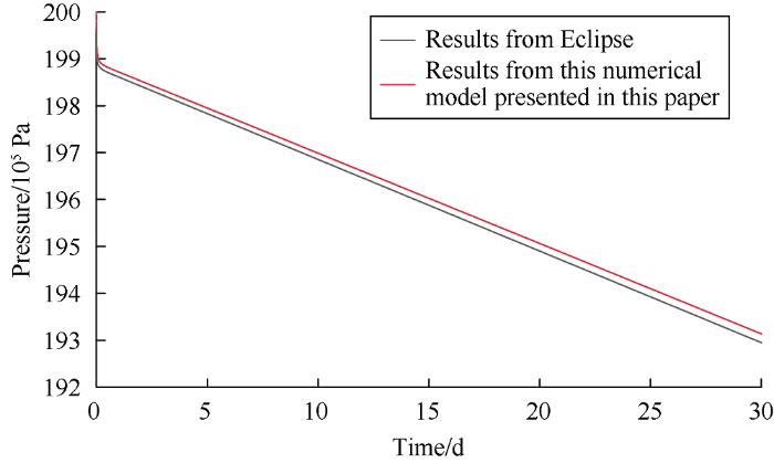
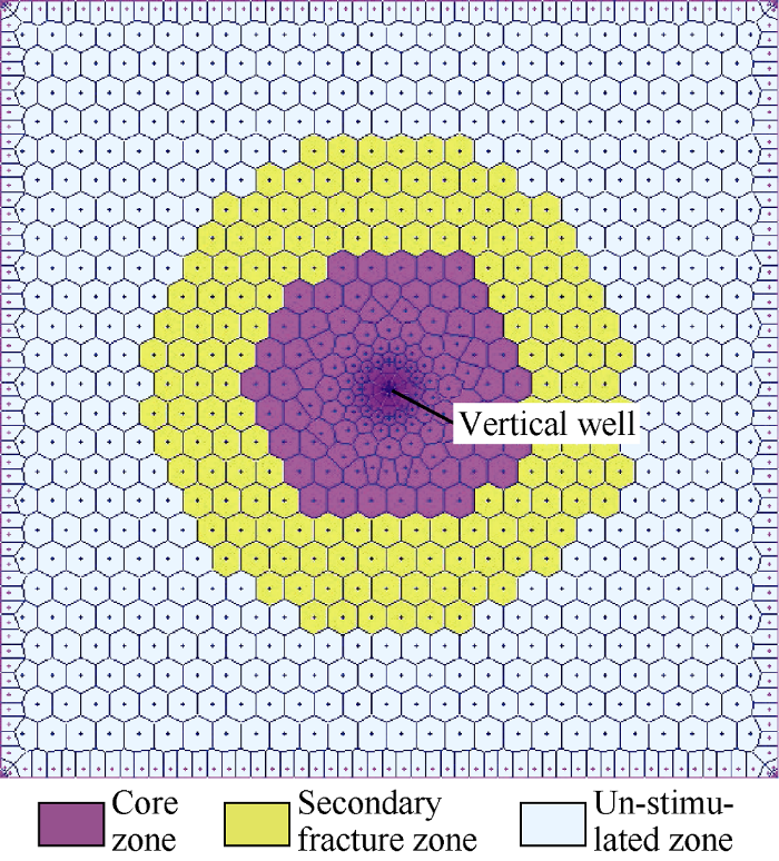
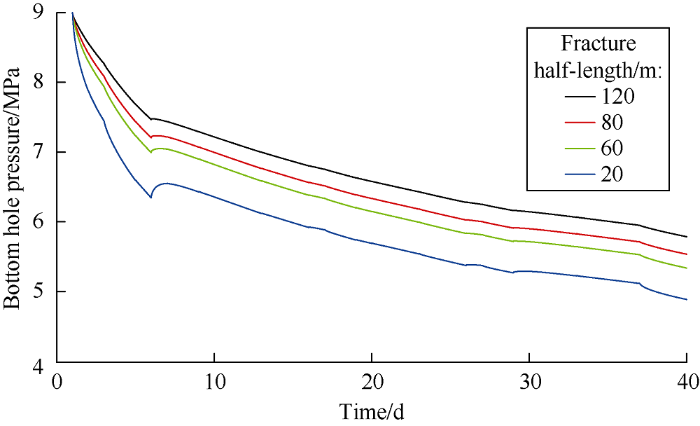
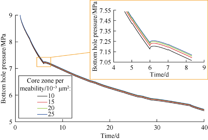
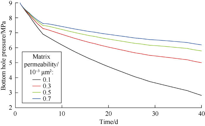
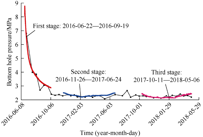
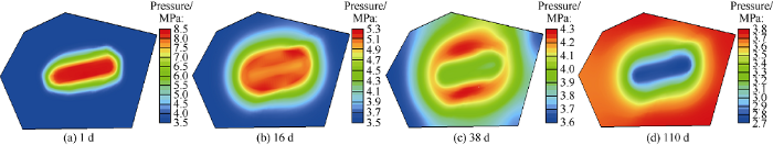
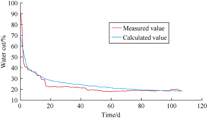

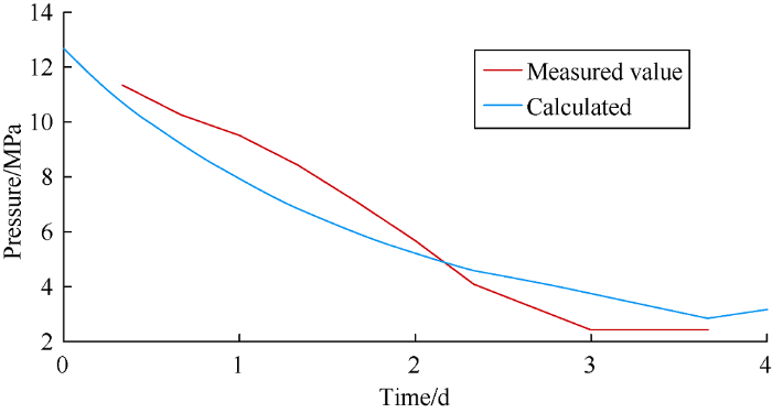
