National Science and Technology Major Project. 2017ZX05009005-002
Abstract
An automatic well test interpretation method for radial composite reservoirs based on convolutional neural network (CNN) is proposed, and its effectiveness and accuracy are verified by actual field data. In this paper, based on the data transformed by logarithm function and the loss function of mean square error (MSE), the optimal CNN is obtained by reducing the loss function to optimize the network with "dropout" method to avoid over fitting. The trained optimal network can be directly used to interpret the buildup or drawdown pressure data of the well in the radial composite reservoir, that is, the log-log plot of the given measured pressure variation and its derivative data are input into the network, the outputs are corresponding reservoir parameters (mobility ratio, storativity ratio, dimensionless composite radius, and dimensionless group characterizing well storage and skin effects), which realizes the automatic initial fitting of well test interpretation parameters. The method is verified with field measured data of Daqing Oilfield. The research shows that the method has high interpretation accuracy, and it is superior to the analytical method and the least square method.
LI Daolun, LIU Xuliang, ZHA Wenshu, YANG Jinghai, LU Detang. Automatic well test interpretation based on convolutional neural network for a radial composite reservoir. [J], 2020, 47(3): 623-631 doi:10.1016/S1876-3804(20)60079-9
Introduction
The artificial intelligence (AI) method has attracted special attention from researchers in the oil industry due to its outstanding performance in handling highly complex problems[1,2,3,4]. Traditional artificial neural network method (ANN) has been widely used in the field of petroleum engineering. Li et al.[5] used implicit method of ANN to predict the log data of unknown years, and then proposed a method for time series processing by combination of implicit curve and neural network[6]. Asadisaghandi et al.[7] used ANN to predict the pressure-volume-temperature (PVT) of oil. Enab et al.[8] developed forward and inverse ANN to predict gas recovery profile, etc. Singh et al.[9] estimated the porosity with ANN technique. Memon et al.[10] constructed the dynamic well Surrogate Reservoir Model (SRM) by radial basis neural network to predict the bottom hole flowing pressure. Kim et al.[11] proposed an approach based on ANN to select completion mode for shale gas reservoirs. Recently, Choubineh et al.[12] estimated the minimum miscible pressure of gas-crude oil by using neural network models.
Since the 1990s, the traditional ANNs have been applied in well test interpretation. Athichanagorn et al.[13] used ANN to identify the features of the derivative plot. Deng et al.[14] used peak value and horizontal position of radial flow in derivative plot as the input of three-layer feedforward neural network to predict well test parameters. Jeirani et al.[15] inputted Horner plot into neural network to estimate reservoir pressure, permeability and skin factor. Adibifard et al.[16] took the coefficients of interpolation Chebyshev polynomials of pressure derivative data as the input of ANN to estimate reservoir parameters. Ghaffarian et al.[17] identified the gas condensate reservoir model by using the pseudo-pressure derivative data as the input of single and coupled multi-layer perceptron network. However, the well test interpretation method based on traditional ANN has the following problems. First, taking a part of characteristics of pressure derivative curve as the input of ANN makes it difficult to realize true automatic well test interpretation. For example, only coefficients of Chebyshev polynomial are taken as input of network[16]. Secondly, the well test curves are complex and changeable, which require a large amount of data to train the network. However, traditional 3-layer or 4-layer networks often fail in training the big data volume, limiting the improvement of its automatic interpretation.
Deep learning (DL) is a new field in machine learning. The essence of deep learning is to build network model with multiple hidden layers, and to obtain more representative features by learning large amount of data, thereby to improve the accuracy of prediction and classification. In recent years, deep learning has also been applied to the oil industry. Tian et al.[18] used recursive neural network to learn permanent downhole pressure gauge (PDG) data for reservoir model identification and production prediction. Sudakov et al.[19] applied deep learning to permeability prediction. ZHA et al.[20] used deep learning to reconstruct porous media. Zhang et al.[21] studied the generation and repair of logging curves by recurrent neural network. Convolutional neural network (CNN) is an important part of deep learning algorithm. It differs from traditional ANNs in the following aspects: (1) CNNs break the limitations of traditional ANNs on the number of layers, increase the number of network layers and forming deep network; (2) CNNs adopt the method of feature learning and extract feature layer by layer to make the prediction or classification more easy to realize. Research on CNNs began in the 1980s. Time-delay network and LeNet-5 network were the earliest CNN algorithms[22,23]. In the 21st century, with the introduction of deep learning theory, the increase of data volume, and the improvement of computing equipment, CNNs have developed rapidly. The AlexNet network proposed by Krizhevsky et al.[24] has been widely used, and later CNNs have been applied in the oil industry[25].
Based on CNN, an automatic well test interpretation approach for radial composite reservoir has been proposed in this work. By this method, the formation parameters can be interpreted by inputting pressure change and derivative into the network, without manual parameter adjustment and fitting, realizing automatic interpretation. The effectiveness and accuracy of this method were verified by the field measurement data of Daqing Oilfield.
1. Summary of the method
1.1. Radial composite reservoir model and well test interpretation parameters
The radial composite reservoir model is composed of two regions with different parameter attributes, namely, a circular inner zone with the well-centered and an infinite outer zone. The radial composite reservoir model can describe pollution or stimulation of the zone around well, change of radial lithology and fluid property in the zone far from the well. The basic assumptions of the radial composite reservoir model are as follows: (1) The formation is horizontal, equal in thickness, homogeneous and isotropic. (2) The fluids in both the inner and outer zones are slightly compressible single-phase fluids and their flow obeys the Darcy's law. (3) The pressure is equal everywhere in the formation before the well is opened. (4) The effect of wellbore storage and wellbore pollution are considered, but gravity is ignored.
The well test curve used in this study is Gringarten-Bourdet composite curve, which is composed of Gringarten pressure curve and Bourdet pressure derivative curve[26,27]. Considering the universality, the method proposed adopts dimensionless parameters. Therefore, the well test interpretation parameters of the radial composite reservoir model include: mobility ratio M, storage ratio F, dimensionless composite radius RfD and dimensionless group CDe2S. The parameters are transformed into logarithmic forms of lg(M), lg(F), lg(RfD) and lg(CDe2S). The dimensionless group characterizes well storage and skin effect. The dimensionless composite radius is defined as:
Convolutional neural network is a kind of deep feed-forward neural network. It is mainly composed of input layer, convolutional layer, pooling layer, fully connected layer and output layer. There are usually several convolutional layers. The pooling layer is located behind the convolutional layer. The fully connected layer is usually at the end of the network. The activation function follows the convolutional and fully connected layer to add non-linearity to the network. The convolution operation is performed between the input data and convolution kernel in the convolution layer, and is usually indicated by the sign “*”. Let f(x) and g(x) be two integrable functions in the real number field, then their convolution results are:
$ f\left( x \right)*g\left( x \right)=\int_{-\infty }^{\infty }{f\left( \tau \right)g\left( x-\tau \right)\text{d}\tau }$
The convolution result of number sequence x(n) and h(n) is:
$ x\left( n \right)*h\left( n \right)=\sum\limits_{s=-\infty }^{\infty }{x\left( s \right)h\left( n-s \right)}$
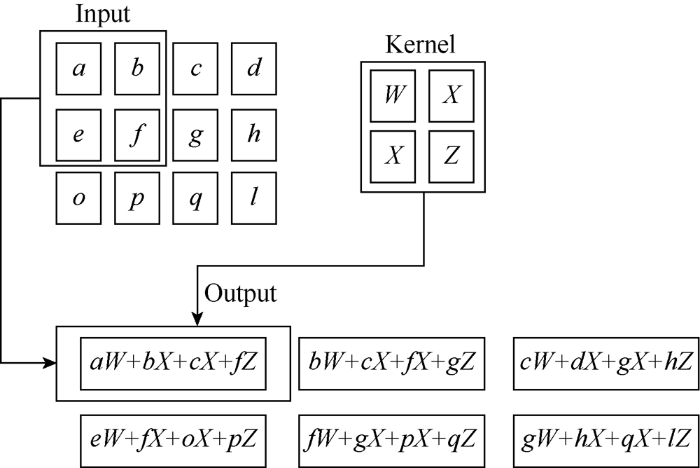
The input of convolution layer and convolutional kernel are usually multidimensional array data. Convolutional operation is actually the sliding process of the kernel over the input of convolutional layer. Multiply the neurons value on the kernel by the corresponding value on input data and the multiplied values are added up as an inactive neuron of next layer. For example, given a 2D input xij and a 2D kernel fuv, where 1≤i≤N1, 1≤j≤N2, 1≤u≤n1, 1≤v≤n2. Generally, n1≤N1, n2≤N2. In this case, the convolution result is:
Different from the traditional neural network, convolution operation improves the network performance through two important characteristics: local connection and weight sharing. The traditional ANN usually adopts matrix multiplication to construct the connection between input and output, this kind of connection is full connection, which means that each output neuron is connected with each input neuron. But CNNs have the feature of local connection, that is, each output is connected to a part of the input, which greatly reduces the number of parameters and makes the network easy to train. The local connection makes the neuron perceive only the local area, and the lower level local area information is integrated to obtain global information at the higher level, which greatly enhances the network feature extraction capability. Each connection has a different weight in full connection. However, in the convolution layer, rather than having different weights, connections in a set can share the same network weight. Local connection and weight sharing make CNN far superior to traditional ANN in statistical efficiency and storage requirements. There are 18 convolution layers in the network in this paper with matrix of 100×100 as input. The network only has 590 688 parameters. If the full connection mode is adopted with 200 neurons in each hidden layer, 2.621 44×1045 parameters would be generated from the input to the 18th hidden layer, far more than the number of parameters using convolution operation.
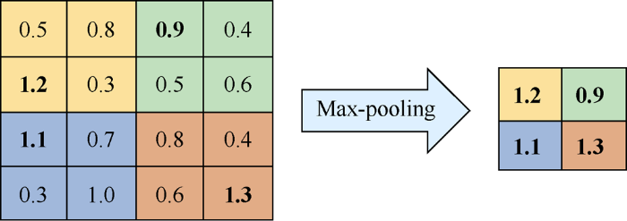
Pooling, also known as down sampling, extracts the overall characteristic of the adjacent region of a location as the output, and thus reduces the amount of data, characteristic dimensions and network parameters. The common pooling methods are max-pooling and average-pooling. Max-pooling takes the maximum characteristic value of the adjacent areas, while average-pooling takes the average characteristic value of the points in adjacent areas. Fig. 2 shows an example of max- pooling. The network input in this paper is a matrix of 100× 100, which becomes the matrix of 50×50 after the first layer of pooling layer, greatly reducing the feature dimension and making the network easier to train.
Fig. 2.
An example of max-pooling (select the maximum value in 2×2 rectangular area).
It can be seen that compared with the traditional ANNs, CNNs have fewer parameters, easier training, more efficient feature extraction, and much better learning ability and performance.
1.3. Automatic well test interpretation method based on CNN
The detailed steps of the automatic well test interpretation method based on CNN are as follows.
(1) Data collection and preprocessing. Artificial intelligence is a kind of data science, CNN is no exception. In this study, a total of 2×10⁵ log-log plots of radial composite reservoir and their corresponding reservoir parameter combinations lg(M), lg(F), lg(RfD), and lg(CDe2S) were obtained, of which 199 820 sets were generated by the analytical method, the rest were field measured data. When generating the simulation data, the value ranges of the parameters are shown in Table 1.
Table 1
Table 1Parameter value ranges during simulation data generation.
The pressure change and derivative curve in each simulated log-log plot consist of 200 data points. However, the actual field plots usually have 100 to 110 data points in each curve. In order to maintain the consistency of the input dimensions, 100 consecutive data points were selected in each iterative training.
In practical applications, CNN is usually used for object recognition and its input is the pixel values of the image, which is a 2D or 3D matrix. Therefore, before training, the log-log plot data needs to be converted into matrix: for each log-log plot, the 100 pressure data and 100 pressure derivative data points were copied and connected together to form a matrix of 100×100.
(2) Training and optimization of CNN. The matrix in step (1) and corresponding parameter combinations lg(M), lg(F), lg(RfD), and lg(CDe2S) were used as the input and output of CNN respectively. 90%, 5% and 5% of the data were used for training, verification and testing respectively. The loss function was mean square error (MSE). The MSE is calculated as:
$ MSE=\frac{1}{N}\sum\limits_{k=1}^{N}{\left\{ {{\left[ {{d}_{1}}\left( k \right)-{{y}_{1}}\left( k \right) \right]}^{2}}\text{+}{{\left[ {{d}_{2}}\left( k \right)-{{y}_{2}}\left( k \right) \right]}^{2}}\text{+} \right.}$ $\left. {{\left[ {{d}_{\text{3}}}\left( k \right)-{{y}_{\text{3}}}\left( k \right) \right]}^{2}}\text{+}{{\left[ {{d}_{\text{4}}}\left( k \right)-{{y}_{\text{4}}}\left( k \right) \right]}^{2}} \right\}$
The smaller the MSE of the training data, the better the network fitting result is. The network was optimized through repeated experiments, and optimization process includes changing network depth, width, super parameters, etc, and adding the regularization method or other methods. The optimal network configuration is obtained through optimization at last. The optimal CNN obtained in this study consists of 18 convolution layers, 3 pooling layers and 3 fully connected layers. The outputs of each convolution layer and full connection layer were activated by ReLU (linear rectification function). The output value of the ReLU function is the maximum value between the independent variable and zero, which makes the output of some neurons zero, increasing the network sparsity and reducing the training time. The network adopted the "dropout" method[24], which set the output of each hidden neuron to zero at a certain probability in forward propagation to avoid overfitting. The initial learning rate was 0.0001. In order to make the model more stable in the later stages of training, this study used exponential decay method to gradually reduce learning rate during each iterative training.
(3) The trained optimal network was used for automatic initial fitting of well test parameter interpretation. The measured pressure data was transformed into log-log plot, then rearranged into a matrix, input into the trained optimal CNN, the output were lg(M), lg(F), lg(RfD), and lg(CDe2S), and then M, F, RfD and CDe2S were obtained, realizing the automatic initial fitting of well test interpretation parameters.
(4) Move curves and explain the wellbore and formation parameters. The typical curve was obtained by inputting M, F, RfD and CDe2S into the commercial software, and the typical curve was moved to make it coincide with the measured log-log plot. Take any point from the measured curve, record the pressure change value Δp and time value t of the point, and find out the dimensionless pressure change value pD and dimensionless time value tD on typical curve at this point. With values of Δp, t, pD and tD of this point and parameters M, F, RfD and CDe2S, wellbore storage coefficient, skin coefficient, permeability of inner and outer zones and other wellbore and reservoir parameters can be calculated according to a series of formulas[29].
2. Results and discussion
2.1. Differences between the method presented in this paper and artificial neural network-based methods
In the method presented in this paper, the pressure change and its derivative data are directly taken as the input of the network. In the previous methods based on artificial neural networks, the inputs are some characteristics obtained from the pressure change and its derivative data. For example, Deng et al.[14] used the hump value of derivative plot and the horizontal position of radial flow as the inputs of neural network. Adibifard et al.[16] took the coefficient of interpolation Chebyshev polynomial as the network input.
2.2. Performance verification of CNN
The validation set and test set data were used to verify the interpretation accuracy of the optimal trained CNN. Table 2 presents the mean absolute errors (MAEs) of the interpretation values for the validation and test sets. It can be seen all the four reservoir parameters have small average absolute errors, indicating that the network is well trained and has good generalization ability.
Table 2
Table 2MAEs of interpretation values of validation set and test set data (the absolute value of absolute error is taken).
In order to exhibit the interpretation effect of the method presented in this paper more clearly, three samples were extracted from the verification set and test set respectively to further demonstrate the performance of the trained CNN. Samples Val1, Val2, and Val3 were taken from the validation set, samples Test1, Test2, and Test3 were taken from the test set. The interpretation results are given in Table 3.
Table 3
Table 3Parameter interpretation values of the 6 samples selected and their absolute errors.
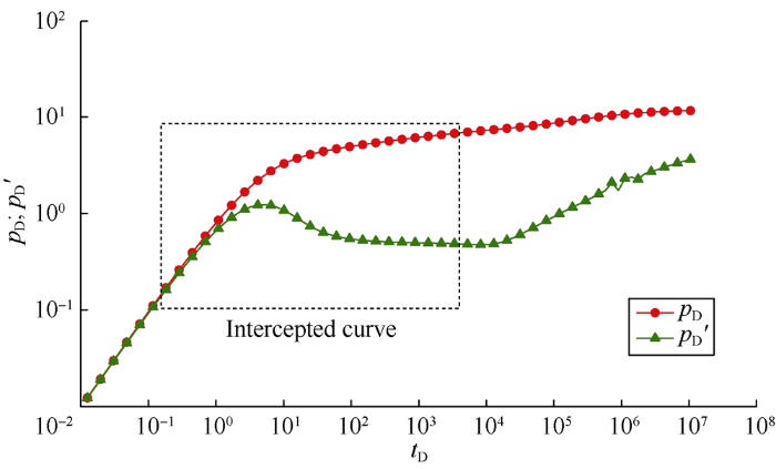
It can be seen from Table 3 that for the six samples, the errors between the interpreted parameters and the real parameters are small on the whole. However, the interpretation errors of lg(F) for sample Val2, lg(M) and lg(CDe2S) for Val3, lg(M), lg(F), and lg(CDe2S) for Test2 are relatively large. The large errors in interpretation values of lg(M) and lg(F) are mainly caused by data intercepting errors, as not all features were intercepted, the interpretation results are poor. The sample Test2 is taken as an example to explain the reason in details. The original and intercepted curves of the Test2 are shown in Fig. 3. It can be seen that the curve intercepted during the test doesn’t include the upwarping part of late stage in the original curve, and this part of curve is the key to characterize the mobility ratio and storage ratio. This is the reason for the poor interpretation effect of the mobility ratio and storage ratio.
Fig. 3.
Original and intercepted curves of sample Test 2.
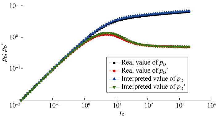
Although the absolute error of the parameter lg(CDe2S) of the sample Test2 is relatively large, its relative error is only 0.167 5. Fig. 4 shows that the early stage of the two log-log plots obtained from the interpreted values and the real values almost coincide, which indicates the interpretation error is small.
Fig. 4.
Comparison of interpreted and actual values of the sample Test2 (only the early stage of curves are taken).
2.3. Analysis of field cases
The validity of the method presented in this paper was further verified by six field cases from Daqing Oilfield. Table 4 presents the basic parameters of the 6 field cases.
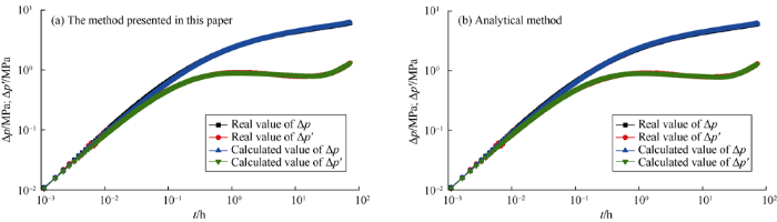
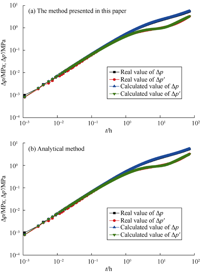
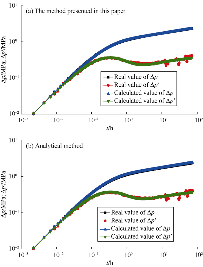
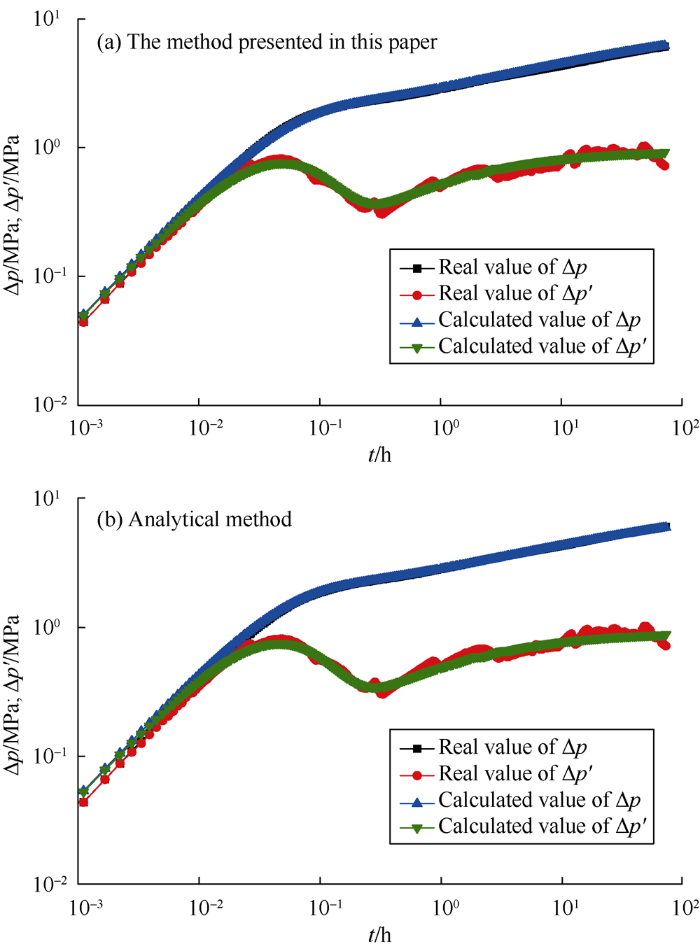
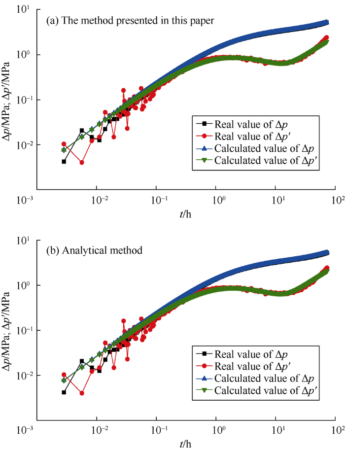
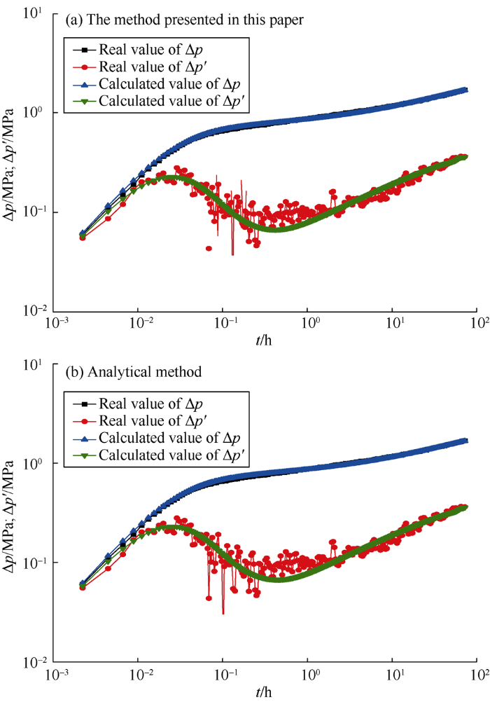
Fig. 5 to Fig. 10 show the comparison of calculation results between the method presented in this paper and analytical method. Table 5 gives the corresponding interpretation parameters. It can be seen from Fig. 5a and Fig. 6a that for the measured data without noise or with slight noise, the method presented in this paper can correctly interpret the parameters, which can be seen from the near coincidence of the measured and the calculated curves. As the noise increases, as shown in Fig. 7a and Fig. 8a, the interpretation results are still good. Even when the measured data has clutter noise, the trained CNN can still explain the formation and wellbore parameters quite accurately (Fig. 9a). Even when the measured data oscillate up and down locally, Fig. 10a illustrates that the interpretation result is still good. It is proved that this method has good effectiveness and robustness. Even if there are some “bad samples” in the training samples, the trained CNN can still correctly interpret the shut-in pressure data. This indicates that a small number of "bad samples" would not affect the performance of the CNN, but the corresponding parameters of “bad samples” couldn’t be interpreted. If the “bad samples” are removed, the CNN after training would have better performance. How to tick out the “bad samples” will be a study content in the future.
In addition, through comparison with analytical method, it is found that the differences between the interpretation results of the method presented in this paper and analytical method are small, and both methods can get good interpretation results. But the analytical method requires professional well testing personnel to complete the operation and costs a lot of manual labor and time. In contrast, the method proposed in this paper can realize automatic interpretation by transforming the measured data into matrix and inputting it into the trained CNN. The outputs are the interpretation parameters. A person without professional knowledge can accomplish well test interpretation aided by the method presented in this paper, which improves work efficiency significantly.
It can be seen that the proposed well test interpretation method based on CNN can interpret radial composite reservoir parameters with high accuracy and efficiency, and realize automatic interpretation of well test data.
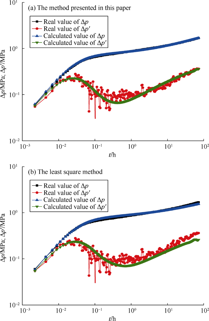
2.4. Comparison between the proposed method and the least square method
Two most representative examples (Case 1 and Case 6) were selected to compare the results from the proposed method and the least square method. The Case 1 has little noise, while Case 6 has a lot of noise. It can be seen from Fig. 11, Fig. 12 and Table 6, the results obtained by the least squares method are poorer. Furthermore, the least square method involves the selection of fitting parameters, so full automatic interpretation can’t be realized by this method.
An automatic well test interpretation method based on CNN for radial composite reservoirs is proposed. By taking the pressure change and derivative data as inputs and the corresponding parameter combinations as outputs, the trained CNN can automatically interpret the pressure data and give the parameters of radial composite reservoir. This method can realize automatic fitting of well test parameters and improve the efficiency of well test interpretation. Its effectiveness and robustness have been verified by the measured data of Daqing Oilfield, and this method has been proved superior to analytical method and the least square method by cases of Daqing Oilfield.
This method can’t be simply copied to other types of reservoirs. As different types of reservoirs differ widely in characteristics of well test curves and the number of parameters, different neural network structures and related processing methods are needed.
Nomenclature
B—volume factor, m3/m3;
C—wellbore storage coefficient, m3/MPa;
CD—dimensionless wellbore storage coefficient;
Ct—total compressibility factor, Pa-1;
d1(k), d2(k), d3(k), d4(k)—interpreted values of lg(M), lg(F), lg(RfD) and lg(CDe2S) in the k-th parameter combination;
fuv—2D convolution kernel;
f(x), g(x)—function;
F—storage ratio, dimensionless;
h(n), x(n)—number sequence;
H—formation thickness, m;
i, j—row and column numbers of 2D input;
K—permeability, 10-3 μm2;
M—mobility ratio, dimensionless;
MSE—mean square error;
n, s—length of number sequence;
n1, n2—the number of rows and columns of 2D convolution kernel;
N—number of parameter combinations;
N1, N2—number of rows and columns of 2D input;
pD—dimensionless pressure change, pD=2πKHΔp/QBμ;
pD'—dimensionless derivative of pressure change, pD'=tDdpD/dtD;
Δp—pressure change, MPa;
Δp'—derivative of pressure change, Δp'=ΔtdΔp/dΔt, MPa;
Q—production, m3/s;
rw—wellbore radius, m;
Rf—composite radius, m;
RfD—dimensionless composite radius;
S—skin factor, dimensionless;
t—time, h;
Δt—time change, h;
tD—dimensionless time, tD=Kt/fμCtrw2;
u, v—row and column numbers of convolution kernel;
x, τ—independent variables of function;
xij—2D input;
y1(k), y2(k), y3(k), y4(k)—real values of lg(M), lg(F), lg(RfD) and lg(CDe2S) in the k-th parameter combination;
Comparative evaluation of back-propagation neural network learning algorithms and empirical correlations for prediction of oil PVT properties in Iran oilfields
Journal of Petroleum Science & Engineering, 2011,78(2):464-475.
Estimation of minimum miscibility pressure of varied gas compositions and reservoir crude oil over a wide range of conditions using an artificial neural network model
Artificial Neural Network (ANN) is used to estimate reservoir parameters from well test data. Theoretical pressure derivative curves, generated by the Sthefest numerical Laplace inverse algorithm and belonged to a Naturally Fractured Reservoir (NFR) with Pseudo Steady State (PSS) inetrporosity flow, used to train the ANN. Instead of using normalized pressure derivative data as ANN's input, the coefficients of interpolating Chebysehv polynomials on the pressure derivative data in log-log plot were used as input to the ANN. Different training algorithms used to train the ANN and optimum number of neurons for each algorithm were obtained through minimizing Mean Relative Error (MRE) over test data. According to the results of MRE, it is concluded that Levenberg-Marquardt algorithm has the lowest possible MRE among various training algorithms used to train the ANN. In order to compare the accuracy of the new proposed method with the previously used methods, normalized pressure derivative data and coefficients of the conventional polynomials are used to train the ANN. Results show that employing the coefficients of the Chebyshev polynomials as input to ANN's decreases MRE over test data while using coefficients of conventional polynomials worsens learning phase of the neural network compared to the normalization method. The lower values of the MRE when using conventional polynomials arise from the fact that interpolating a function using Chebyshev polynomials is more accurate than other interpolation techniques for a specific number of basic functions. Test data are used to verify the accuracy of the trained ANN to estimate each reservoir parameter. Low relative error values of reservoir parameters when using test data shows the capability of the new method which employs the Chebyshev polynomial coefficients as input to train ANN. Moreover, a field data for a dual-porosity fractured reservoir is applied to make a comparison of ANN's outputs with the results obtained using different well test softwares and normalization method. The results show a good consistency between ANN and well test softwares. (C) 2014 Elsevier B.V.
GHAFFARIANN, ESLAMLOEYANR, VAFERIB.
Model identification for gas condensate reservoirs by using ANN method based on well test data
Journal of Petroleum Science and Engineering, 2014,123:20-29.
ImageNet classification with deep convolutional neural networks: Proceedings of the 25th International Conference on Neural Information Processing Systems
New York: Curran Associates Inc., 2012: 1097-1105.
Reservoir simulation and modeling based on artificial intelligence and data mining (AI & DM)
1
2011
... The artificial intelligence (AI) method has attracted special attention from researchers in the oil industry due to its outstanding performance in handling highly complex problems[1,2,3,4]. Traditional artificial neural network method (ANN) has been widely used in the field of petroleum engineering. Li et al.[5] used implicit method of ANN to predict the log data of unknown years, and then proposed a method for time series processing by combination of implicit curve and neural network[6]. Asadisaghandi et al.[7] used ANN to predict the pressure-volume-temperature (PVT) of oil. Enab et al.[8] developed forward and inverse ANN to predict gas recovery profile, etc. Singh et al.[9] estimated the porosity with ANN technique. Memon et al.[10] constructed the dynamic well Surrogate Reservoir Model (SRM) by radial basis neural network to predict the bottom hole flowing pressure. Kim et al.[11] proposed an approach based on ANN to select completion mode for shale gas reservoirs. Recently, Choubineh et al.[12] estimated the minimum miscible pressure of gas-crude oil by using neural network models. ...
Full field reservoir modeling of shale assets using advanced data-driven analytics
1
2016
... The artificial intelligence (AI) method has attracted special attention from researchers in the oil industry due to its outstanding performance in handling highly complex problems[1,2,3,4]. Traditional artificial neural network method (ANN) has been widely used in the field of petroleum engineering. Li et al.[5] used implicit method of ANN to predict the log data of unknown years, and then proposed a method for time series processing by combination of implicit curve and neural network[6]. Asadisaghandi et al.[7] used ANN to predict the pressure-volume-temperature (PVT) of oil. Enab et al.[8] developed forward and inverse ANN to predict gas recovery profile, etc. Singh et al.[9] estimated the porosity with ANN technique. Memon et al.[10] constructed the dynamic well Surrogate Reservoir Model (SRM) by radial basis neural network to predict the bottom hole flowing pressure. Kim et al.[11] proposed an approach based on ANN to select completion mode for shale gas reservoirs. Recently, Choubineh et al.[12] estimated the minimum miscible pressure of gas-crude oil by using neural network models. ...
Optimization of well placement geothermal reservoirs using artificial intelligence
1
2010
... The artificial intelligence (AI) method has attracted special attention from researchers in the oil industry due to its outstanding performance in handling highly complex problems[1,2,3,4]. Traditional artificial neural network method (ANN) has been widely used in the field of petroleum engineering. Li et al.[5] used implicit method of ANN to predict the log data of unknown years, and then proposed a method for time series processing by combination of implicit curve and neural network[6]. Asadisaghandi et al.[7] used ANN to predict the pressure-volume-temperature (PVT) of oil. Enab et al.[8] developed forward and inverse ANN to predict gas recovery profile, etc. Singh et al.[9] estimated the porosity with ANN technique. Memon et al.[10] constructed the dynamic well Surrogate Reservoir Model (SRM) by radial basis neural network to predict the bottom hole flowing pressure. Kim et al.[11] proposed an approach based on ANN to select completion mode for shale gas reservoirs. Recently, Choubineh et al.[12] estimated the minimum miscible pressure of gas-crude oil by using neural network models. ...
Application of artificial intelligence to forecast hydrocarbon production from shales
1
2018
... The artificial intelligence (AI) method has attracted special attention from researchers in the oil industry due to its outstanding performance in handling highly complex problems[1,2,3,4]. Traditional artificial neural network method (ANN) has been widely used in the field of petroleum engineering. Li et al.[5] used implicit method of ANN to predict the log data of unknown years, and then proposed a method for time series processing by combination of implicit curve and neural network[6]. Asadisaghandi et al.[7] used ANN to predict the pressure-volume-temperature (PVT) of oil. Enab et al.[8] developed forward and inverse ANN to predict gas recovery profile, etc. Singh et al.[9] estimated the porosity with ANN technique. Memon et al.[10] constructed the dynamic well Surrogate Reservoir Model (SRM) by radial basis neural network to predict the bottom hole flowing pressure. Kim et al.[11] proposed an approach based on ANN to select completion mode for shale gas reservoirs. Recently, Choubineh et al.[12] estimated the minimum miscible pressure of gas-crude oil by using neural network models. ...
Processing of well log data based on backpropagation neural network implicit approximation
1
2007
... The artificial intelligence (AI) method has attracted special attention from researchers in the oil industry due to its outstanding performance in handling highly complex problems[1,2,3,4]. Traditional artificial neural network method (ANN) has been widely used in the field of petroleum engineering. Li et al.[5] used implicit method of ANN to predict the log data of unknown years, and then proposed a method for time series processing by combination of implicit curve and neural network[6]. Asadisaghandi et al.[7] used ANN to predict the pressure-volume-temperature (PVT) of oil. Enab et al.[8] developed forward and inverse ANN to predict gas recovery profile, etc. Singh et al.[9] estimated the porosity with ANN technique. Memon et al.[10] constructed the dynamic well Surrogate Reservoir Model (SRM) by radial basis neural network to predict the bottom hole flowing pressure. Kim et al.[11] proposed an approach based on ANN to select completion mode for shale gas reservoirs. Recently, Choubineh et al.[12] estimated the minimum miscible pressure of gas-crude oil by using neural network models. ...
Implicit approximation of neural network and applications
1
2009
... The artificial intelligence (AI) method has attracted special attention from researchers in the oil industry due to its outstanding performance in handling highly complex problems[1,2,3,4]. Traditional artificial neural network method (ANN) has been widely used in the field of petroleum engineering. Li et al.[5] used implicit method of ANN to predict the log data of unknown years, and then proposed a method for time series processing by combination of implicit curve and neural network[6]. Asadisaghandi et al.[7] used ANN to predict the pressure-volume-temperature (PVT) of oil. Enab et al.[8] developed forward and inverse ANN to predict gas recovery profile, etc. Singh et al.[9] estimated the porosity with ANN technique. Memon et al.[10] constructed the dynamic well Surrogate Reservoir Model (SRM) by radial basis neural network to predict the bottom hole flowing pressure. Kim et al.[11] proposed an approach based on ANN to select completion mode for shale gas reservoirs. Recently, Choubineh et al.[12] estimated the minimum miscible pressure of gas-crude oil by using neural network models. ...
Comparative evaluation of back-propagation neural network learning algorithms and empirical correlations for prediction of oil PVT properties in Iran oilfields
1
2011
... The artificial intelligence (AI) method has attracted special attention from researchers in the oil industry due to its outstanding performance in handling highly complex problems[1,2,3,4]. Traditional artificial neural network method (ANN) has been widely used in the field of petroleum engineering. Li et al.[5] used implicit method of ANN to predict the log data of unknown years, and then proposed a method for time series processing by combination of implicit curve and neural network[6]. Asadisaghandi et al.[7] used ANN to predict the pressure-volume-temperature (PVT) of oil. Enab et al.[8] developed forward and inverse ANN to predict gas recovery profile, etc. Singh et al.[9] estimated the porosity with ANN technique. Memon et al.[10] constructed the dynamic well Surrogate Reservoir Model (SRM) by radial basis neural network to predict the bottom hole flowing pressure. Kim et al.[11] proposed an approach based on ANN to select completion mode for shale gas reservoirs. Recently, Choubineh et al.[12] estimated the minimum miscible pressure of gas-crude oil by using neural network models. ...
Artificial neural network based design for dual lateral well applications
1
2014
... The artificial intelligence (AI) method has attracted special attention from researchers in the oil industry due to its outstanding performance in handling highly complex problems[1,2,3,4]. Traditional artificial neural network method (ANN) has been widely used in the field of petroleum engineering. Li et al.[5] used implicit method of ANN to predict the log data of unknown years, and then proposed a method for time series processing by combination of implicit curve and neural network[6]. Asadisaghandi et al.[7] used ANN to predict the pressure-volume-temperature (PVT) of oil. Enab et al.[8] developed forward and inverse ANN to predict gas recovery profile, etc. Singh et al.[9] estimated the porosity with ANN technique. Memon et al.[10] constructed the dynamic well Surrogate Reservoir Model (SRM) by radial basis neural network to predict the bottom hole flowing pressure. Kim et al.[11] proposed an approach based on ANN to select completion mode for shale gas reservoirs. Recently, Choubineh et al.[12] estimated the minimum miscible pressure of gas-crude oil by using neural network models. ...
A general approach for porosity estimation using artificial neural network method: A case study from Kansas gas field
1
2015
... The artificial intelligence (AI) method has attracted special attention from researchers in the oil industry due to its outstanding performance in handling highly complex problems[1,2,3,4]. Traditional artificial neural network method (ANN) has been widely used in the field of petroleum engineering. Li et al.[5] used implicit method of ANN to predict the log data of unknown years, and then proposed a method for time series processing by combination of implicit curve and neural network[6]. Asadisaghandi et al.[7] used ANN to predict the pressure-volume-temperature (PVT) of oil. Enab et al.[8] developed forward and inverse ANN to predict gas recovery profile, etc. Singh et al.[9] estimated the porosity with ANN technique. Memon et al.[10] constructed the dynamic well Surrogate Reservoir Model (SRM) by radial basis neural network to predict the bottom hole flowing pressure. Kim et al.[11] proposed an approach based on ANN to select completion mode for shale gas reservoirs. Recently, Choubineh et al.[12] estimated the minimum miscible pressure of gas-crude oil by using neural network models. ...
Dynamic well bottom-hole flowing pressure prediction based on radial basis neural network
1
2015
... The artificial intelligence (AI) method has attracted special attention from researchers in the oil industry due to its outstanding performance in handling highly complex problems[1,2,3,4]. Traditional artificial neural network method (ANN) has been widely used in the field of petroleum engineering. Li et al.[5] used implicit method of ANN to predict the log data of unknown years, and then proposed a method for time series processing by combination of implicit curve and neural network[6]. Asadisaghandi et al.[7] used ANN to predict the pressure-volume-temperature (PVT) of oil. Enab et al.[8] developed forward and inverse ANN to predict gas recovery profile, etc. Singh et al.[9] estimated the porosity with ANN technique. Memon et al.[10] constructed the dynamic well Surrogate Reservoir Model (SRM) by radial basis neural network to predict the bottom hole flowing pressure. Kim et al.[11] proposed an approach based on ANN to select completion mode for shale gas reservoirs. Recently, Choubineh et al.[12] estimated the minimum miscible pressure of gas-crude oil by using neural network models. ...
A comprehensive approach to select completion and fracturing fluid in shale gas reservoirs using the artificial neural network
1
2017
... The artificial intelligence (AI) method has attracted special attention from researchers in the oil industry due to its outstanding performance in handling highly complex problems[1,2,3,4]. Traditional artificial neural network method (ANN) has been widely used in the field of petroleum engineering. Li et al.[5] used implicit method of ANN to predict the log data of unknown years, and then proposed a method for time series processing by combination of implicit curve and neural network[6]. Asadisaghandi et al.[7] used ANN to predict the pressure-volume-temperature (PVT) of oil. Enab et al.[8] developed forward and inverse ANN to predict gas recovery profile, etc. Singh et al.[9] estimated the porosity with ANN technique. Memon et al.[10] constructed the dynamic well Surrogate Reservoir Model (SRM) by radial basis neural network to predict the bottom hole flowing pressure. Kim et al.[11] proposed an approach based on ANN to select completion mode for shale gas reservoirs. Recently, Choubineh et al.[12] estimated the minimum miscible pressure of gas-crude oil by using neural network models. ...
Estimation of minimum miscibility pressure of varied gas compositions and reservoir crude oil over a wide range of conditions using an artificial neural network model
1
2019
... The artificial intelligence (AI) method has attracted special attention from researchers in the oil industry due to its outstanding performance in handling highly complex problems[1,2,3,4]. Traditional artificial neural network method (ANN) has been widely used in the field of petroleum engineering. Li et al.[5] used implicit method of ANN to predict the log data of unknown years, and then proposed a method for time series processing by combination of implicit curve and neural network[6]. Asadisaghandi et al.[7] used ANN to predict the pressure-volume-temperature (PVT) of oil. Enab et al.[8] developed forward and inverse ANN to predict gas recovery profile, etc. Singh et al.[9] estimated the porosity with ANN technique. Memon et al.[10] constructed the dynamic well Surrogate Reservoir Model (SRM) by radial basis neural network to predict the bottom hole flowing pressure. Kim et al.[11] proposed an approach based on ANN to select completion mode for shale gas reservoirs. Recently, Choubineh et al.[12] estimated the minimum miscible pressure of gas-crude oil by using neural network models. ...
Automatic parameter estimation from well test data using artificial neural network
1
1995
... Since the 1990s, the traditional ANNs have been applied in well test interpretation. Athichanagorn et al.[13] used ANN to identify the features of the derivative plot. Deng et al.[14] used peak value and horizontal position of radial flow in derivative plot as the input of three-layer feedforward neural network to predict well test parameters. Jeirani et al.[15] inputted Horner plot into neural network to estimate reservoir pressure, permeability and skin factor. Adibifard et al.[16] took the coefficients of interpolation Chebyshev polynomials of pressure derivative data as the input of ANN to estimate reservoir parameters. Ghaffarian et al.[17] identified the gas condensate reservoir model by using the pseudo-pressure derivative data as the input of single and coupled multi-layer perceptron network. However, the well test interpretation method based on traditional ANN has the following problems. First, taking a part of characteristics of pressure derivative curve as the input of ANN makes it difficult to realize true automatic well test interpretation. For example, only coefficients of Chebyshev polynomial are taken as input of network[16]. Secondly, the well test curves are complex and changeable, which require a large amount of data to train the network. However, traditional 3-layer or 4-layer networks often fail in training the big data volume, limiting the improvement of its automatic interpretation. ...
Using artificial neural network to realize type curve match analysis of well test data
2
2000
... Since the 1990s, the traditional ANNs have been applied in well test interpretation. Athichanagorn et al.[13] used ANN to identify the features of the derivative plot. Deng et al.[14] used peak value and horizontal position of radial flow in derivative plot as the input of three-layer feedforward neural network to predict well test parameters. Jeirani et al.[15] inputted Horner plot into neural network to estimate reservoir pressure, permeability and skin factor. Adibifard et al.[16] took the coefficients of interpolation Chebyshev polynomials of pressure derivative data as the input of ANN to estimate reservoir parameters. Ghaffarian et al.[17] identified the gas condensate reservoir model by using the pseudo-pressure derivative data as the input of single and coupled multi-layer perceptron network. However, the well test interpretation method based on traditional ANN has the following problems. First, taking a part of characteristics of pressure derivative curve as the input of ANN makes it difficult to realize true automatic well test interpretation. For example, only coefficients of Chebyshev polynomial are taken as input of network[16]. Secondly, the well test curves are complex and changeable, which require a large amount of data to train the network. However, traditional 3-layer or 4-layer networks often fail in training the big data volume, limiting the improvement of its automatic interpretation. ...
... In the method presented in this paper, the pressure change and its derivative data are directly taken as the input of the network. In the previous methods based on artificial neural networks, the inputs are some characteristics obtained from the pressure change and its derivative data. For example, Deng et al.[14] used the hump value of derivative plot and the horizontal position of radial flow as the inputs of neural network. Adibifard et al.[16] took the coefficient of interpolation Chebyshev polynomial as the network input. ...
Estimating the initial pressure, permeability and skin factor of oil reservoirs using artificial neural networks
1
2006
... Since the 1990s, the traditional ANNs have been applied in well test interpretation. Athichanagorn et al.[13] used ANN to identify the features of the derivative plot. Deng et al.[14] used peak value and horizontal position of radial flow in derivative plot as the input of three-layer feedforward neural network to predict well test parameters. Jeirani et al.[15] inputted Horner plot into neural network to estimate reservoir pressure, permeability and skin factor. Adibifard et al.[16] took the coefficients of interpolation Chebyshev polynomials of pressure derivative data as the input of ANN to estimate reservoir parameters. Ghaffarian et al.[17] identified the gas condensate reservoir model by using the pseudo-pressure derivative data as the input of single and coupled multi-layer perceptron network. However, the well test interpretation method based on traditional ANN has the following problems. First, taking a part of characteristics of pressure derivative curve as the input of ANN makes it difficult to realize true automatic well test interpretation. For example, only coefficients of Chebyshev polynomial are taken as input of network[16]. Secondly, the well test curves are complex and changeable, which require a large amount of data to train the network. However, traditional 3-layer or 4-layer networks often fail in training the big data volume, limiting the improvement of its automatic interpretation. ...
Artificial Neural Network (ANN) to estimate reservoir parameters in Naturally Fractured Reservoirs using well test data
3
2014
... Since the 1990s, the traditional ANNs have been applied in well test interpretation. Athichanagorn et al.[13] used ANN to identify the features of the derivative plot. Deng et al.[14] used peak value and horizontal position of radial flow in derivative plot as the input of three-layer feedforward neural network to predict well test parameters. Jeirani et al.[15] inputted Horner plot into neural network to estimate reservoir pressure, permeability and skin factor. Adibifard et al.[16] took the coefficients of interpolation Chebyshev polynomials of pressure derivative data as the input of ANN to estimate reservoir parameters. Ghaffarian et al.[17] identified the gas condensate reservoir model by using the pseudo-pressure derivative data as the input of single and coupled multi-layer perceptron network. However, the well test interpretation method based on traditional ANN has the following problems. First, taking a part of characteristics of pressure derivative curve as the input of ANN makes it difficult to realize true automatic well test interpretation. For example, only coefficients of Chebyshev polynomial are taken as input of network[16]. Secondly, the well test curves are complex and changeable, which require a large amount of data to train the network. However, traditional 3-layer or 4-layer networks often fail in training the big data volume, limiting the improvement of its automatic interpretation. ...
... [16]. Secondly, the well test curves are complex and changeable, which require a large amount of data to train the network. However, traditional 3-layer or 4-layer networks often fail in training the big data volume, limiting the improvement of its automatic interpretation. ...
... In the method presented in this paper, the pressure change and its derivative data are directly taken as the input of the network. In the previous methods based on artificial neural networks, the inputs are some characteristics obtained from the pressure change and its derivative data. For example, Deng et al.[14] used the hump value of derivative plot and the horizontal position of radial flow as the inputs of neural network. Adibifard et al.[16] took the coefficient of interpolation Chebyshev polynomial as the network input. ...
Model identification for gas condensate reservoirs by using ANN method based on well test data
1
2014
... Since the 1990s, the traditional ANNs have been applied in well test interpretation. Athichanagorn et al.[13] used ANN to identify the features of the derivative plot. Deng et al.[14] used peak value and horizontal position of radial flow in derivative plot as the input of three-layer feedforward neural network to predict well test parameters. Jeirani et al.[15] inputted Horner plot into neural network to estimate reservoir pressure, permeability and skin factor. Adibifard et al.[16] took the coefficients of interpolation Chebyshev polynomials of pressure derivative data as the input of ANN to estimate reservoir parameters. Ghaffarian et al.[17] identified the gas condensate reservoir model by using the pseudo-pressure derivative data as the input of single and coupled multi-layer perceptron network. However, the well test interpretation method based on traditional ANN has the following problems. First, taking a part of characteristics of pressure derivative curve as the input of ANN makes it difficult to realize true automatic well test interpretation. For example, only coefficients of Chebyshev polynomial are taken as input of network[16]. Secondly, the well test curves are complex and changeable, which require a large amount of data to train the network. However, traditional 3-layer or 4-layer networks often fail in training the big data volume, limiting the improvement of its automatic interpretation. ...
Recurrent neural networks for permanent downhole gauge data analysis
1
2017
... Deep learning (DL) is a new field in machine learning. The essence of deep learning is to build network model with multiple hidden layers, and to obtain more representative features by learning large amount of data, thereby to improve the accuracy of prediction and classification. In recent years, deep learning has also been applied to the oil industry. Tian et al.[18] used recursive neural network to learn permanent downhole pressure gauge (PDG) data for reservoir model identification and production prediction. Sudakov et al.[19] applied deep learning to permeability prediction. ZHA et al.[20] used deep learning to reconstruct porous media. Zhang et al.[21] studied the generation and repair of logging curves by recurrent neural network. Convolutional neural network (CNN) is an important part of deep learning algorithm. It differs from traditional ANNs in the following aspects: (1) CNNs break the limitations of traditional ANNs on the number of layers, increase the number of network layers and forming deep network; (2) CNNs adopt the method of feature learning and extract feature layer by layer to make the prediction or classification more easy to realize. Research on CNNs began in the 1980s. Time-delay network and LeNet-5 network were the earliest CNN algorithms[22,23]. In the 21st century, with the introduction of deep learning theory, the increase of data volume, and the improvement of computing equipment, CNNs have developed rapidly. The AlexNet network proposed by Krizhevsky et al.[24] has been widely used, and later CNNs have been applied in the oil industry[25]. ...
Driving digital rock towards machine learning: Predicting permeability with gradient boosting and deep neural networks
1
2019
... Deep learning (DL) is a new field in machine learning. The essence of deep learning is to build network model with multiple hidden layers, and to obtain more representative features by learning large amount of data, thereby to improve the accuracy of prediction and classification. In recent years, deep learning has also been applied to the oil industry. Tian et al.[18] used recursive neural network to learn permanent downhole pressure gauge (PDG) data for reservoir model identification and production prediction. Sudakov et al.[19] applied deep learning to permeability prediction. ZHA et al.[20] used deep learning to reconstruct porous media. Zhang et al.[21] studied the generation and repair of logging curves by recurrent neural network. Convolutional neural network (CNN) is an important part of deep learning algorithm. It differs from traditional ANNs in the following aspects: (1) CNNs break the limitations of traditional ANNs on the number of layers, increase the number of network layers and forming deep network; (2) CNNs adopt the method of feature learning and extract feature layer by layer to make the prediction or classification more easy to realize. Research on CNNs began in the 1980s. Time-delay network and LeNet-5 network were the earliest CNN algorithms[22,23]. In the 21st century, with the introduction of deep learning theory, the increase of data volume, and the improvement of computing equipment, CNNs have developed rapidly. The AlexNet network proposed by Krizhevsky et al.[24] has been widely used, and later CNNs have been applied in the oil industry[25]. ...
Reconstruction of shale image based on Wasserstein Generative Adversarial Networks with gradient penalty
1
2020
... Deep learning (DL) is a new field in machine learning. The essence of deep learning is to build network model with multiple hidden layers, and to obtain more representative features by learning large amount of data, thereby to improve the accuracy of prediction and classification. In recent years, deep learning has also been applied to the oil industry. Tian et al.[18] used recursive neural network to learn permanent downhole pressure gauge (PDG) data for reservoir model identification and production prediction. Sudakov et al.[19] applied deep learning to permeability prediction. ZHA et al.[20] used deep learning to reconstruct porous media. Zhang et al.[21] studied the generation and repair of logging curves by recurrent neural network. Convolutional neural network (CNN) is an important part of deep learning algorithm. It differs from traditional ANNs in the following aspects: (1) CNNs break the limitations of traditional ANNs on the number of layers, increase the number of network layers and forming deep network; (2) CNNs adopt the method of feature learning and extract feature layer by layer to make the prediction or classification more easy to realize. Research on CNNs began in the 1980s. Time-delay network and LeNet-5 network were the earliest CNN algorithms[22,23]. In the 21st century, with the introduction of deep learning theory, the increase of data volume, and the improvement of computing equipment, CNNs have developed rapidly. The AlexNet network proposed by Krizhevsky et al.[24] has been widely used, and later CNNs have been applied in the oil industry[25]. ...
Synthetic well logs generation via Recurrent Neural Networks
1
2018
... Deep learning (DL) is a new field in machine learning. The essence of deep learning is to build network model with multiple hidden layers, and to obtain more representative features by learning large amount of data, thereby to improve the accuracy of prediction and classification. In recent years, deep learning has also been applied to the oil industry. Tian et al.[18] used recursive neural network to learn permanent downhole pressure gauge (PDG) data for reservoir model identification and production prediction. Sudakov et al.[19] applied deep learning to permeability prediction. ZHA et al.[20] used deep learning to reconstruct porous media. Zhang et al.[21] studied the generation and repair of logging curves by recurrent neural network. Convolutional neural network (CNN) is an important part of deep learning algorithm. It differs from traditional ANNs in the following aspects: (1) CNNs break the limitations of traditional ANNs on the number of layers, increase the number of network layers and forming deep network; (2) CNNs adopt the method of feature learning and extract feature layer by layer to make the prediction or classification more easy to realize. Research on CNNs began in the 1980s. Time-delay network and LeNet-5 network were the earliest CNN algorithms[22,23]. In the 21st century, with the introduction of deep learning theory, the increase of data volume, and the improvement of computing equipment, CNNs have developed rapidly. The AlexNet network proposed by Krizhevsky et al.[24] has been widely used, and later CNNs have been applied in the oil industry[25]. ...
Phoneme recognition using time-delay neural networks
1
1987
... Deep learning (DL) is a new field in machine learning. The essence of deep learning is to build network model with multiple hidden layers, and to obtain more representative features by learning large amount of data, thereby to improve the accuracy of prediction and classification. In recent years, deep learning has also been applied to the oil industry. Tian et al.[18] used recursive neural network to learn permanent downhole pressure gauge (PDG) data for reservoir model identification and production prediction. Sudakov et al.[19] applied deep learning to permeability prediction. ZHA et al.[20] used deep learning to reconstruct porous media. Zhang et al.[21] studied the generation and repair of logging curves by recurrent neural network. Convolutional neural network (CNN) is an important part of deep learning algorithm. It differs from traditional ANNs in the following aspects: (1) CNNs break the limitations of traditional ANNs on the number of layers, increase the number of network layers and forming deep network; (2) CNNs adopt the method of feature learning and extract feature layer by layer to make the prediction or classification more easy to realize. Research on CNNs began in the 1980s. Time-delay network and LeNet-5 network were the earliest CNN algorithms[22,23]. In the 21st century, with the introduction of deep learning theory, the increase of data volume, and the improvement of computing equipment, CNNs have developed rapidly. The AlexNet network proposed by Krizhevsky et al.[24] has been widely used, and later CNNs have been applied in the oil industry[25]. ...
Gradient-based learning applied to document recognition
1
1998
... Deep learning (DL) is a new field in machine learning. The essence of deep learning is to build network model with multiple hidden layers, and to obtain more representative features by learning large amount of data, thereby to improve the accuracy of prediction and classification. In recent years, deep learning has also been applied to the oil industry. Tian et al.[18] used recursive neural network to learn permanent downhole pressure gauge (PDG) data for reservoir model identification and production prediction. Sudakov et al.[19] applied deep learning to permeability prediction. ZHA et al.[20] used deep learning to reconstruct porous media. Zhang et al.[21] studied the generation and repair of logging curves by recurrent neural network. Convolutional neural network (CNN) is an important part of deep learning algorithm. It differs from traditional ANNs in the following aspects: (1) CNNs break the limitations of traditional ANNs on the number of layers, increase the number of network layers and forming deep network; (2) CNNs adopt the method of feature learning and extract feature layer by layer to make the prediction or classification more easy to realize. Research on CNNs began in the 1980s. Time-delay network and LeNet-5 network were the earliest CNN algorithms[22,23]. In the 21st century, with the introduction of deep learning theory, the increase of data volume, and the improvement of computing equipment, CNNs have developed rapidly. The AlexNet network proposed by Krizhevsky et al.[24] has been widely used, and later CNNs have been applied in the oil industry[25]. ...
ImageNet classification with deep convolutional neural networks: Proceedings of the 25th International Conference on Neural Information Processing Systems
2
2012
... Deep learning (DL) is a new field in machine learning. The essence of deep learning is to build network model with multiple hidden layers, and to obtain more representative features by learning large amount of data, thereby to improve the accuracy of prediction and classification. In recent years, deep learning has also been applied to the oil industry. Tian et al.[18] used recursive neural network to learn permanent downhole pressure gauge (PDG) data for reservoir model identification and production prediction. Sudakov et al.[19] applied deep learning to permeability prediction. ZHA et al.[20] used deep learning to reconstruct porous media. Zhang et al.[21] studied the generation and repair of logging curves by recurrent neural network. Convolutional neural network (CNN) is an important part of deep learning algorithm. It differs from traditional ANNs in the following aspects: (1) CNNs break the limitations of traditional ANNs on the number of layers, increase the number of network layers and forming deep network; (2) CNNs adopt the method of feature learning and extract feature layer by layer to make the prediction or classification more easy to realize. Research on CNNs began in the 1980s. Time-delay network and LeNet-5 network were the earliest CNN algorithms[22,23]. In the 21st century, with the introduction of deep learning theory, the increase of data volume, and the improvement of computing equipment, CNNs have developed rapidly. The AlexNet network proposed by Krizhevsky et al.[24] has been widely used, and later CNNs have been applied in the oil industry[25]. ...
... The smaller the MSE of the training data, the better the network fitting result is. The network was optimized through repeated experiments, and optimization process includes changing network depth, width, super parameters, etc, and adding the regularization method or other methods. The optimal network configuration is obtained through optimization at last. The optimal CNN obtained in this study consists of 18 convolution layers, 3 pooling layers and 3 fully connected layers. The outputs of each convolution layer and full connection layer were activated by ReLU (linear rectification function). The output value of the ReLU function is the maximum value between the independent variable and zero, which makes the output of some neurons zero, increasing the network sparsity and reducing the training time. The network adopted the "dropout" method[24], which set the output of each hidden neuron to zero at a certain probability in forward propagation to avoid overfitting. The initial learning rate was 0.0001. In order to make the model more stable in the later stages of training, this study used exponential decay method to gradually reduce learning rate during each iterative training. ...
Deep learning convolutional neural networks to predict porous media properties
1
2018
... Deep learning (DL) is a new field in machine learning. The essence of deep learning is to build network model with multiple hidden layers, and to obtain more representative features by learning large amount of data, thereby to improve the accuracy of prediction and classification. In recent years, deep learning has also been applied to the oil industry. Tian et al.[18] used recursive neural network to learn permanent downhole pressure gauge (PDG) data for reservoir model identification and production prediction. Sudakov et al.[19] applied deep learning to permeability prediction. ZHA et al.[20] used deep learning to reconstruct porous media. Zhang et al.[21] studied the generation and repair of logging curves by recurrent neural network. Convolutional neural network (CNN) is an important part of deep learning algorithm. It differs from traditional ANNs in the following aspects: (1) CNNs break the limitations of traditional ANNs on the number of layers, increase the number of network layers and forming deep network; (2) CNNs adopt the method of feature learning and extract feature layer by layer to make the prediction or classification more easy to realize. Research on CNNs began in the 1980s. Time-delay network and LeNet-5 network were the earliest CNN algorithms[22,23]. In the 21st century, with the introduction of deep learning theory, the increase of data volume, and the improvement of computing equipment, CNNs have developed rapidly. The AlexNet network proposed by Krizhevsky et al.[24] has been widely used, and later CNNs have been applied in the oil industry[25]. ...
Determination of fissure volume and block size in fractured reservoirs by type-curve analysis
1
1980
... The well test curve used in this study is Gringarten-Bourdet composite curve, which is composed of Gringarten pressure curve and Bourdet pressure derivative curve[26,27]. Considering the universality, the method proposed adopts dimensionless parameters. Therefore, the well test interpretation parameters of the radial composite reservoir model include: mobility ratio M, storage ratio F, dimensionless composite radius RfD and dimensionless group CDe2S. The parameters are transformed into logarithmic forms of lg(M), lg(F), lg(RfD) and lg(CDe2S). The dimensionless group characterizes well storage and skin effect. The dimensionless composite radius is defined as: ...
New type curves aid analysis of fissured zone well tests
1
1984
... The well test curve used in this study is Gringarten-Bourdet composite curve, which is composed of Gringarten pressure curve and Bourdet pressure derivative curve[26,27]. Considering the universality, the method proposed adopts dimensionless parameters. Therefore, the well test interpretation parameters of the radial composite reservoir model include: mobility ratio M, storage ratio F, dimensionless composite radius RfD and dimensionless group CDe2S. The parameters are transformed into logarithmic forms of lg(M), lg(F), lg(RfD) and lg(CDe2S). The dimensionless group characterizes well storage and skin effect. The dimensionless composite radius is defined as: ...
1
2016
... Fig. 1 shows an example of a 2D array convolution[28]. ...
Well test analysis: The use of advanced interpretation models
1
2002
... (4) Move curves and explain the wellbore and formation parameters. The typical curve was obtained by inputting M, F, RfD and CDe2S into the commercial software, and the typical curve was moved to make it coincide with the measured log-log plot. Take any point from the measured curve, record the pressure change value Δp and time value t of the point, and find out the dimensionless pressure change value pD and dimensionless time value tD on typical curve at this point. With values of Δp, t, pD and tD of this point and parameters M, F, RfD and CDe2S, wellbore storage coefficient, skin coefficient, permeability of inner and outer zones and other wellbore and reservoir parameters can be calculated according to a series of formulas[29]. ...


