


Introduction
With the revolution of shale oil and gas technology in the United States, unconventional oil and gas resources have become the main development targets[1,2,3]. As a core technology of development, the multi-stage fracturing technology for long horizontal wells has been widely recognized and applied both at home and abroad. But there is still a common industrial problem in horizontal well development: how to optimize the length of horizontal section, the number of artificial fractures, the fracture spacing, the section length of fracturing, the number of clusters inside the section, the number of perforations in each cluster to reach the goal of slowing down production decline and enhancing recovery rate. Aiming at these problems, after years of studies, the authors have come up with a new method of reservoir stimulation for horizontal well: fracture-controlling fracturing (FCF) technology[4].
The FCF technology is to achieve the maximum production of reserves in the well-controlled unit through the optimization of artificial fracture parameters. For the conventional vertical well fracturing, the relevant dimension parameters of bilateral symmetrical fractures including the half-fracture length, fracture height, fracture width and artificial fracture conductivity adaptable to the formation need to be optimized, to obtain the maximum production and maximum recovery rate of reserves in the controlled unit of vertical wells. For horizontal wells with more artificial fractures and more complex initiation and expansion of fractures, the fracture-controlling fracturing technology involves optimizing the relevant parameters such as fracture orientation, fracture dimensions (length, width and height), space between fractures in the controlled production units of the horizontal wells and the row space of horizontal wells, as well as on-site operation process parameters simultaneously to achieve the maximum production of the controlled unit, the maximum recovery rate and optimal economic benefit of the horizontal wells.
The FCF technology is a complex systematic engineering, which involves the description of the reservoirs in the well control unit, the characteristics of seepage flow of the fluids as well as the shape of a single hydraulic fracture; the characterization of the relationship between artificial fracture density and reservoir physical properties and the relationship between the rock mechanical properties and in-situ stress; the influence of various parameters on the life cycle development of unconventional reservoirs, etc.
From the development of the fracturing technology and the trend of the present grade changes of the proven hydrocarbon resources, the FCF technology is expected to become the main fracturing technology[5,6,7,8]. The means of its implementation are as follows: (1) Developing geology-engineering integrated fracturing optimal design software to optimize the fracture system and achieve optimal control over the hydrocarbon resources in low-grade reservoirs; (2) developing a high efficiency multifunction fracturing fluid system to maximize the stimulation, energy storage, imbibition and displacement functions of the fracturing fluid; (3) emphasizing the application of large-scale low-cost stimulation technologies in site operation to strive to achieve the purpose of stimulation in the initial completion. The FCF technology is further merged into the development of low-grade hydrocarbon resources and can be upgraded as the main development mode for unconventional resources. This paper briefly introduces the software optimization model, applicability of fracture controlling fracturing technology, principles and methods for optimal design, and field tests completed.
1. Key points of FCF technology
The core of the FCF technology is to optimize fracturing design. Establishing an optimization model and developing the corresponding software are the basis of the technology. At present, the bridge plug staged & multi-cluster perforation mode fracturing is generally adopted for more than 90% unconventional horizontal wells[9]. Therefore, the optimal model of the FCF must be able to achieve: (1) multi-stage induced fracture stimulation in horizontal wells for developing unconventional reservoirs; (2) oil-gas reservoir production simulation under the condition of large-scale fracturing.
1.1. Propagation model of multiple fractures in a horizontal well
A full-3D fracture propagation model is adopted to simulate the propagation of multiple fractures in horizontal wells multi-stage and multi-cluster fracturing[10,11]. The model does not consider the distribution of natural fractures and the interaction between natural fractures and artificial fractures. The hydraulic fractures are described as continuously distributed main fractures[12,13,14]. It is assumed that the fractures remain vertical[15] (the minimum principal stress in most tight oil and shale gas reservoirs in China is horizontal, and hydraulic fracturing often results in vertical fractures) but can expand in any horizontal direction. The fractures are composed of a series of structured rectangular elements, with the main variables (pressure and fracture width, etc.) located at the central nodes of the elements. The size of the vertical fracture element can be adjusted automatically to accurately match the thickness of different layers, while the element size of the horizontal fracture remains unchanged to improve the calculation efficiency. Specifically, the three-dimensional displacement discontinuity method is adopted to describe the fracture opening and shear deformation and finally build the elastic equation:
The fluid flow in the fracture meets the mass conservation equation:
The momentum equations of the fluid motion are as follows:
The fluid loss is defined by one-dimensional Carter leak-off model:
Equation (1) describing fracture deformation and Equation (2) representing the equation of mass conservation for fluid flow in the fractures jointly constitute a group of transient nonlinear coupled equations with fracture width and fluid pressure as unknowns. For Equation (2) of the mass conservation equation, the finite volume method is used for discretization. The coupled equations are solved with the method of sequential coupling analysis: (1) The given time step is $\Delta t$ and the distribution of fluid pressure $p$in the fractures and fracture width$w$for the last time step are known. Assuming that the initial flow distributed in each cluster (pump injection displacement in fracture point source) is ${{q}_{i}}$ and it meets the volume conservation rule. (2) Equation (2) is adopted to calculate the fracture width $w$ of the current time step and the fracture width is substituted into Equation (1) to calculate the discontinuous quantities of pressure$p$and shear displacement. (3) Substitute the pressure$p$and fracture width $w$ back into Equation (2) to recalculate the fracture width, and make such iteration until the pressure and fracture width are convergent. (4) Calculate the flow distribution in each cluster through the intra-fracture pressure $p$obtained and compare it with the assumed initial flow ${{q}_{i}}$distributed. If they are convergent, the calculation is completed; If not convergent, then redistribute the flow in each cluster and repeat steps (2)-(4). When the maximum tensile stress of the leading edge of the fracture is greater than the tensile strength of the rock, the fracture begins to expand. The direction of fracture propagation is calculated using the stress field to ensure that the direction of local minimum principal stress is always perpendicular to the direction of fracture propagation.
1.2. Numerical simulation model for tight oil & gas reservoir fracturing
In large-scale fracturing of horizontal well in tight oil & gas reservoirs, the interaction between the fracturing fluid and the formation needs to be considered. Previous studies have found that fracturing fluids with specific functions enable more wetting phase to enter the reservoir matrix and displace the non-wetting phase in the reservoir matrix into the fractures. In this process, the fracturing fluid mainly works in two ways to displace oil in the reservoir[16,17]: (1) reducing the interfacial tension between the crude oil in small pore throats of the matrix and the surrounding water and making the oil phase movable; (2) changing the wettability of the reservoir matrix to the water-wet direction and increasing the reverse imbibition of the water phase to improve the recovery ratio of reserves in the matrix.
In order to better describe the large-scale fracturing development dynamics of horizontal wells in tight oil and gas reservoirs, the numerical model must consider the following factors: (1) the simultaneous flow of the three fluids: oil, water and fracturing fluid; (2) the coupling between fluid and fluid as well as coupling between fluid and solid; (3) introducing a wettability reversal model and an interfacial tension reduction model.
1.2.1. Oil and water material balance equation
The model assumes that the flow of the fluid conforms to Darcy seepage flow and is isothermal seepage flow; the water component exists in the water phase and the oil component exists in the oil phase; the temperature in the porous medium is constant, and there is no loss of oil and water in the block. Considering the gravity and capillary force, an oil-water material balance equation is established as follows:
1.2.2. Fracturing fluid material balance equation
Auxiliary materials, such as a surfactant is generally added to the fluid for large-scale fracturing in the tight oil reservoir, so the surfactant effect of the fracturing fluid should also be considered. It is assumed in the model that the surfactant is soluble in oil and water and can be adsorbed onto the solid surface of the rocks. The diffusion of the surfactant molecules meets the Fick's Law and the surfactant has a constant density, so the following equation can be established:
1.2.3. Capillary pressure and relative permeability curves
When entering the reservoir matrix, fracturing fluid would cause changes in capillary pressure and relative permeability of the rock. Based on the Brooks-Corey capillary pressure curve, wettability characterization parameters are added to draw capillary pressure and relative permeability curves before and after wettability reversal. The capillary pressure curve can be expressed as follows[18]:
1.2.4. Wettability reversal equation
Considering the changes of rock wettability caused by fracturing fluid getting into the reservoir matrix, based on Fletcher's experimental results[19], the empirical fitting method is adopted to express the wettability changes, namely the contact angle changes, as a time-dependent function:
Similar to the conventional reservoir numerical simulation software, the implicit expression is adopted for the solution of pressure and the explicit expressions for the solutions of saturation and concentration of surfactant (IMPECS)[20]. For the pressure term, the capillary pressure equation is transformed into ${{p}_{\text{w}}}={{p}_{\text{o}}}-{{p}_{\text{c}}}$ and then substituted into Equation (5) to eliminate the pw term. Merging the two-phase equation to obtain the pressure equation, the pressure distribution is solved and substituted into the original equation to explicitly solve the saturation and surfactant concentration equations.
The calculation steps of the model are as follows: (1) input the reservoir parameters to initialize the model, then calculate the relative permeability curve and capillary pressure curve; (2) calculate the oil phase pressure equation with the pressure difference scheme; (3) calculate the fluid saturation equation and the corresponding new capillary pressure equation; (4) carry out the substance balance tests for oil and water phases; (5) if the test results are qualified, the surfactant concentration equation is solved to obtain the new interfacial tension and contact angle corresponding to the surfactant concentration. If the test results aren’t qualified, reduce the time step and repeat the steps (1)-(4); (6) calculate the saturation front, hydrocarbon production, and recovery rate, etc.
1.3. FrSmart Geo-engineering fracturing design optimization software
Based on fracture simulation and fracturing reservoir simulation, the FrSmart Geo-engineering fracturing design optimization software has been developed. With seven key modules (Fig. 1), this software can complete the following tasks: (1) importing geological modeling data to establish a geomechanically model and optimizing fracturing sections; (2) using the numerical reservoir simulation module to optimize space between artificial fractures, fracture length and other parameters; (3) using the fracture simulation module to optimize the operation parameters; (4) using the economic evaluation module to realize optimization of all the key parameters of unconventional resource development; (5) through integrating the functions of big data, field and remote decision-making, the accuracy of input parameters and the rationality of design can be improved.
Fig. 1.
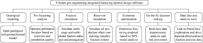
Fig. 1.
Modules and main functions of FrSmart fracturing design optimization software considering geologic and engineering factors.
2. Applicability of the FCF technology
Based on the three grades of resources, extra-low permeability, ultra-low permeability and tight oil reservoirs, in a domestic oilfield as prototypes, the reservoir numerical simulation model presented in this paper was used to calculate and compare the recovery ratios of reserves under different development modes by horizontal and vertical wells, and evaluate the applicability of the FCF technology.
2.1. Basic parameters of modeling
Using the reservoir and fracture parameters shown in Table 1, geological models of the 3 grades of resources, extra-low permeability, ultra-low permeability and tight oil reservoirs were established, which have the same model size of 2500 m×2000 m and mesh size of 25 m×25 m.
Table 1 Main reservoir and fracture parameters in the model.
| Resource grade | Surface crude oil density/ (g•cm-3) | Gas-oil ratio/ (m3•t-1) | In-place oil viscosity/ (mPa•s) | Effective thickness of pay zone/m | Initial reservoir pressure at specified depth/MPa | Depth of given initial reservoir pressure/m | Initial bubble point pressure/MPa |
|---|---|---|---|---|---|---|---|
| Extra-low permeability | 0.763 | 74.3 | 2.24 | 20 | 10.0 | 1 688 | 6.85 |
| Ultra-low permeability | 0.854 | 115.7 | 1.07 | 20 | 16.7 | 2 123 | 12.08 |
| Tight oil | 0.827 | 103.9 | 1.04 | 20 | 16.0 | 1 840 | 7.18 |
| Resource grade | Oil saturation/ % | Effective reservoir permeability/ 10-3 μm2 | Porosity/ % | Injection-production well pattern | Space between producer and injector | Half-fracture length of hydraulic fracturing/m | Dimensionless fracture conductivity |
| Extra-low permeability | 55.9 | 0.230 0 | 12.9 | Square inverted nine-spot | 300×300 m | 135 | 1.5 |
| Ultra-low permeability | 50.0 | 0.080 0 | 12.0 | Diamond inverted nine-spot | 480×130 m | 186 | 2.2 |
| Tight oil | 46.0 | 0.007 5 | 9.0 | Horizontal well depletion pattern | Horizontal interval length 1 500 m | 170 | 3.6 |
2.2. Simulation results
2.2.1. Extra-low permeability reservoir
The development indexes of extra-low permeability reservoirs by the four development modes were calculated by simulation (Fig. 2) : (1) vertical well square inverted nine-spot pattern; (2) vertical well square reverse nine-spot well pattern +in-filling + row water injection (wells were added in the middle of two rows of producers after five years of production to adjust the well pattern into row water injection); (3) depletion development with horizontal wells in 200-m space; (4) depletion development with horizontal wells in 800-m space.
Fig. 2.
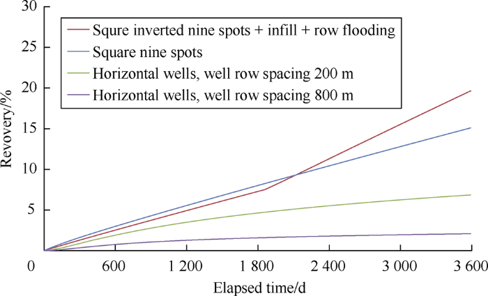
Fig. 2.
Recovery degree of the extra-low permeability reservoir with different development modes.
From the calculation results, it can be seen that: (1) The development mode with a square inverted nine-spot pattern would have a recovery ratio of reserves of 15.3% after 10 years of production. (2) In the development mode in which wells were added to adjust the well pattern into row water injection after 5 years of production when the development effect was the best, the recovery ratio of reserves would reach a maximum of 20.1% after 10 years of production. (3) The depletion development with horizontal wells in 800 m space would have a recovery ratio of only 2.1% after 10 years of production. Even if the row spacing between horizontal wells is reduced to 200 m, the recovery ratio of reserves after 10 years of production would be only 6.9%. (4) By comparing the degrees of producing reserves under different development modes, for the development mode with inverted nine-spot vertical well square pattern, the oil saturation in the side well would decrease by 21.9%, while the oil saturation in the same position under the horizontal well depletion development mode would only decrease by 1.0%, with a very low producing degree. Considering the construction costs of vertical wells and horizontal wells, the extra-low permeability reservoir should be developed with the vertical well inverted nine-spot pattern and then the well pattern can be infilled and adjusted according to the development situation. This is consistent with current oilfield development practices.
2.2.2. Ultra-low permeability reservoir
The development indexes of the ultra-low permeability reservoir under five different development modes were simulated (Fig. 3): (1) vertical well diamond-shaped inverted nine-spot pattern; (2) vertical well square inverted nine-spot pattern; (3) vertical well square inverted nine-spot pattern + in-filling (the infill mode is the same as that of the extra-low permeability reservoir); (4) depletion development with horizontal wells in 200m row space; (5) depletion development with horizontal wells in 800 m row space. According to the simulation results, the development mode with a vertical well square inverted nine-spot pattern would have the highest recovery degree. The economic benefit was considered next. Assuming the horizontal well construction cost is RMB 13 million/well, the construction cost of a vertical well is RMB 1.3 million, and the crude oil price is RMB 3050/t. The development effects and economic benefits under different development modes were calculated as below (Table 2). The results show that the development mode of the square inverted nine-spot pattern has the highest benefit, which is consistent with the current oilfield development practice. Compared with the extra-low permeability reservoir, the gap between the recovery ratio of reserves after 10 years of production with horizontal wells in 200 m space and that with injection and production pattern of vertical wells is narrower. Therefore, it is necessary to explore the feasibility of horizontal well depletion development patterns for ultra-low permeability and difficult reservoirs to establish the relationship between injection and production.
Fig. 3.
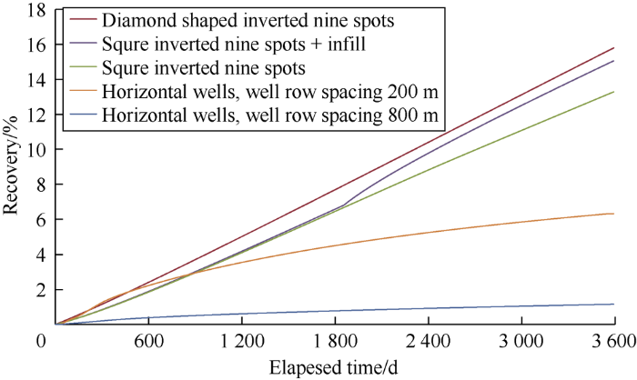
Fig. 3.
Recovery of ultra-low permeability reservoirs under different development modes.
Table 2 Income and recovery ratio of reserves of the ultra-low permeability reservoir under different development modes.
| Development mode | Cumulative oil production/t | Recovery ratio of reserves after 10 years of production/% | Cost/×104RMB | Net income/ ×104RMB |
|---|---|---|---|---|
| Diamond inverted nine-spot | 80 774.5 | 15.9 | 1 170 | 23 468.2 |
| Square inverted nine-spot | 59 511.6 | 13.5 | 1 170 | 16 982.5 |
| Square inverted nine-spot + infilled wells | 66 157.5 | 15.3 | 1 690 | 18 489.7 |
| Horizontal wells in 800 m space | 38 187.5 | 1.3 | 2 600 | 9 048.2 |
| Horizontal well in 200 m space | 46 094.8 | 6.4 | 2 600 | 11 460.1 |
2.2.3. Tight oil
Similarly, the development indexes of the tight oil reservoir under 5 development modes (Fig. 4): (1) vertical well square inverted nine-spot pattern; (2) square inverted nine-spot well pattern + infilled well + row water injection (the infill mode is the same as that for the extra-low permeability reservoir); (3) depletion development with horizontal wells in row space of 200 m; (4) depletion development with horizontal wells in a row space of 400 m; (5) depletion development with horizontal wells in a row space of 800 m, were simulated. It can be seen from the calculation results that due to the extremely poor permeability of the tight oil reservoir, flow channels cannot be established for the injected water, even if the vertical well pattern is infilled, the water flooding effect wouldn’t be seen after 10 years of development. In contrast, depletion development with horizontal wells would have a better effect. When the row space of the horizontal wells is 200 m, the recovery ratio of reserves would be 2.5%. Therefore, the depletion development mode with horizontal wells is suitable for the tight oil reservoir.
Fig. 4.
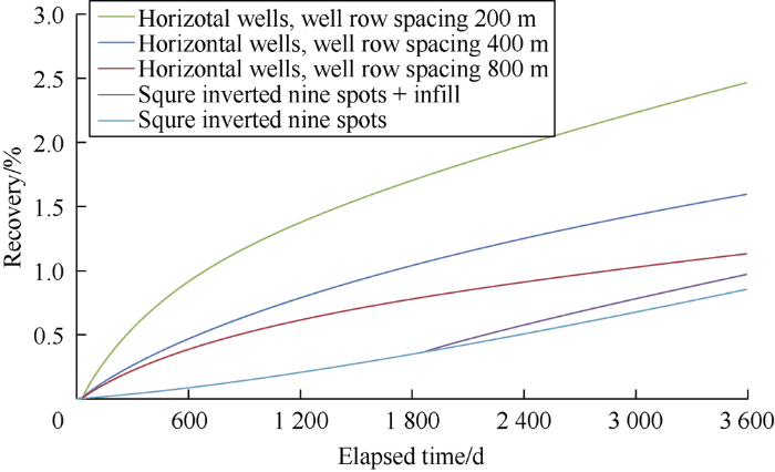
Fig. 4.
Recovery of tight oil reservoirs under different development modes.
Fig. 5 shows the distributions of residual oil saturation after production for 3590 days at different horizontal well row spaces. It can be seen that under the same production time, when the horizontal row space is 200 m, the inter-well oil saturation is the lowest, indicating that reducing the row space between horizontal wells can enhance the degree of oil reserves control, cumulative oil production, and ultimate recovery.
Fig. 5.
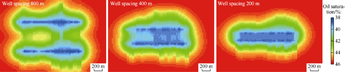
Fig. 5.
Distribution of crude oil saturation at different horizontal well row spacing for developing tight oil reservoirs.
From the above analysis, it can be seen that as the reservoirs get poorer in physical properties, the advantage of horizontal well depletion development stands out gradually. Tight oil reservoirs (with an air permeability of less than 0.1×10⁻³ μm2) have a higher degree of recovery by horizontal well depletion development. The FCF technology can maximize the production of reserves in the well control unit by optimizing the artificial fracture parameters. It is mainly proposed for the horizontal well pattern in depletion development mode, so this technology is suitable for low-grade unconventional resources such as tight oil.
3. Optimization of FCF design for tight oil reservoirs
3.1. Impact of space between induced fractures on production index in horizontal wells
The space between induced fractures in the horizontal well developing tight reservoir was designed as 40, 30, 20, 10, and 5 m, respectively. After inputting the basic data shown in Table 1, FrSmart, the fracturing optimization design software considering both geologic and engineering factors was used to simulate the development indexes of the horizontal wells (Fig. 6). It can be seen from the figure that as the space between fractures reduces, the daily oil production after fracturing increases significantly. According to simulation results, when the space between fractures is 5 m, the cumulative oil production in 3 years would increase by 230% compared with that when the space between fractures is 30 m.
Fig. 6.
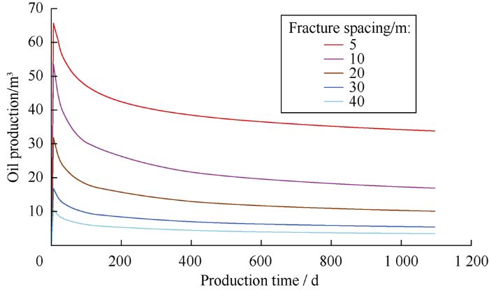
Fig. 6.
Daily oil production under different fracture spacing.
Fig. 7 shows the distributions of oil saturation after three years of production at 20, 10, and 5 m spaces between induced fractures in a horizontal well. The comparison shows that the smaller the space between induced fractures, the lower the residual oil saturation and the higher the degree of producing reserves will be. When the space between fractures is reduced to a certain degree (5 m in this example), the entire reservoir will see even reduction of oil saturation.
Fig. 7.
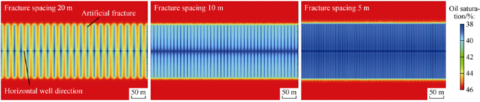
Fig. 7.
Oil saturation distributions under different spacing of fractures.
3.2. Optimization of induced fracture parameters in horizontal wells
The fracture optimization module of the FrSmart software was used to simulate the production performance of horizontal wells under multi-stage and multi-cluster fracturing conditions for the development of the tight oil reservoir to optimize the number of clusters, operation scale, initiation and expansion state of hydraulic fractures. The target horizon of the simulated horizontal well was at the depth of 2385-2415 m. The stress difference between the upper and lower barriers and the target zone was 5-6 MPa. During the simulation, the fracturing length was set as 80m; the same displacement (12 m3/min) and average proppant/liquid ratio (15%) were adopted for all the schemes. See Table 3 and Table 4 for other main basic parameters of the reservoir and the fracturing materials as well as pumping parameters. Three injection volumes, 800, 1600, 2 400 m3 were set for each scheme.
Table 3 Main reservoir and fracturing material parameters for fracture optimization in horizontal well.
| Parameter | Data | Parameter | Data |
|---|---|---|---|
| Horizontal minimum principal stress | 30 MPa | Filtration coefficient | 1.3×10⁻⁴ m/min0.5 |
| Horizontal maximum principal stress | 37 MPa | Hole diameter | 10 mm |
| Young's Modulus | 20 GPa | Slick water viscosity | 5 mPa•s |
| Poisson ratio | 0.25 | Average particle diameter of proppant | 0.15 mm |
| Fracture toughness | 1.5 MPa/m0.5 | Apparent density of proppant | 2 500 kg/m3 |
Table 4 Input parameters of different fracture optimization schemes for horizontal well.
| No. | Number of cluster in one stage | Number of holes in each cluster | Cluster space/m |
|---|---|---|---|
| 1 | 4 | 12 | 20 |
| 2 | 8 | 6 | 10 |
| 3 | 12 | 4 | 7 |
| 4 | 16 | 3 | 5 |
Fig. 8 shows the overhead view and side view of hydraulic fractures of the 4 schemes in Table 4 at the fracturing fluid volume of 1600 m3 for each stage. It can be seen that: (1) With the increase of the number of clusters within one section, and the space between clusters reduces from 20 m to 5 m, the artificial fracture interference intensifies; the artificial fractures in different clusters unevenly expand. (2) As the difference between the two horizontal principal stresses is large (7 MPa), the hydraulic fractures can propagate toward the deeper part of the reservoir. (3) At the same operation scale, when the number of clusters in a stage is 16, the fractures can better control the reservoir to achieve dense cutting of the reservoir.
Fig. 8.
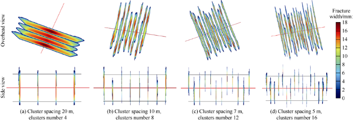
Fig. 8.
Top view and side view of fracture propagation in one stage.
Fig. 9 shows the supported fracture lengths under different operation scales and 8 clusters in one section. There is a non-linear relationship between the fracture length and the operation scale. Increasing unit fracture length in the later stage needs more fracturing materials. For horizontal wells with row spaces of 400 m and 200 m respectively drilled on the same platform: (1) Under the row spacing of 400 m, there are 8 fractures within the segment and the length of each fracture is 200 m. A total of about 3000 m3 fracturing fluid is consumed. (2) Under the row spacing of 200 m, there are 8 fractures within the fragment and the length of each fracture is 100 m. A total of about 1100 m3 fracturing fluid is consumed. The comparison shows that for the same "fracture-controlled" reserves, less fracturing material is consumed by the horizontal wells with a smaller row spacing. To sum up, narrowing horizontal well spacing and thick artificial fractures are the best choices for tight oil reservoirs to achieve fracture control.
Fig. 9.
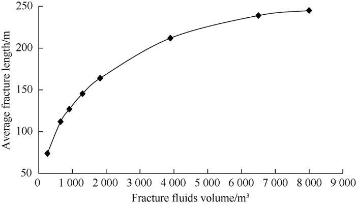
Fig. 9.
Relationship between fracturing fluids and average fracture length.
3.3. Principles for FCF
To achieve the optimum "fracture-controlled" performance, the principles for achieving FCF optimization are proposed as follows: (1) Long horizontal sections of more than 1800 m and a small row space of 200-300 m should be adopted. (2) Fracturing should adopt plug and multi-cluster perforation; the stimulated section should be stable in length (70-100 m), and the number of perforation clusters within one fracturing section (8-16 clusters) should be increased greatly and the space between fractures (5-15 m) should be reduced to achieve the goal of "high-density fracturing". (3) The amount of fracturing fluid and proppant in each section should be optimized. It should be noted if the horizontal well is an infill well, in consideration of the stress drop caused by pressure attenuation, a large amount of fluid should be replenished into the old well before fracturing to reduce mutual interference between the old well and the new well.
4. On-site test of FCF in tight oil reservoirs
The tight oil reservoir in the Chang 7 member of the Ordos Basin is composed of fine and silt grade feldspar debris sandstones, with a core permeability range of (0.11-0.14)×10-3 μm2; horizontal principal stress difference of 4-7 MPa, oil viscosity of 0.97 mPa•s at formation temperature and pressure coefficient of 0.77-0.84.
Since scale production capacity of Chang 7 tight oil built in 2013, the average horizontal section length has increased steadily, the fracturing sections number has increased gradually, and the designed space between fractures has been reduced from 30-40 m to 15 m. Through research using the above optimization method, it is concluded that the designed space between fractures can be reduced to about 5-8 m, so it is necessary to carry out field tests of fracture control fracturing technology to further reduce space between fractures and increase fracture controlled reserves.
In FCF operation, soluble plugs were used to seal different sections, the number of clusters in a section was increased from 4-6 to 12-14. Each cluster had 2 holes at the phase angle of 180°. For a single horizontal well, although the total number of clusters increased significantly, the average fracturing section length and the total sections in a well remained unchanged, so the overall fracturing cost remained stable, making it possible to realize low-cost fracturing.
The first FCF test in the horizontal well was completed in 2019, and the well had a daily fluid production of 25.0 m3 and an average water content of 35.1% after fracturing. In 2019, 87 wells in this block were treated by FCF technology, these wells have a horizontal length of 1705.8 m, 22.3 fracturing section, 118.9 clusters, space between clusters of 10.9 m, and initial output of 18.6 t/d per well on average. Compared with horizontal wells with the same section length, the initial daily oil production after fracturing increased by about 1.5 times, and the single-well forecasted final recovery degree is expected to increase by 44.4%.
5. Conclusions
The vertical well pattern is suitable for the development of extra-low to ultra-low permeability reservoirs. The horizontal well depletion pattern is suitable for the development of tight oil reservoirs. The FCF technology achieves the maximum deployment of reserves in the well control unit through the optimization of artificial fracture parameters. The best application targets of this technology are unconventional oil and gas resources such as tight oil reservoirs.
FCF technology enables the effective development of unconventional oil and gas resources such as tight oil reservoirs. The key points of the FCF include: increasing the length of the horizontal section and reducing the row space between horizontal wells; greatly increasing the number of clusters in a section and reducing the space between fractures; avoiding fracturing interference between old wells and new wells.
Field tests have proved that the FCF technology can improve well productivity and the recovery ratio of reserves. Further integration of the FCF technology with oil and gas field development can greatly improve the development efficiency of unconventional resources such as tight oil fields in China.
Nomenclature
Bo, Bw—volume coefficients of the oil-phase and water-phase fluids, dimensionless;
CL—fluid loss coefficient, m/s0.5;
CMC—critical micelle concentration, mg/mL;
Cp—capillary pressure endpoint coefficient, Pa•m;
Csw, Cso, Csg—surfactant concentrations adsorbed by water phase, oil phase and rock surface, m3/m3;
$C\left( t \right)$—a function of the concentration of surfactant in the aqueous phase over time, mg/mL;
d—experimental data fitting index, dimensionless;
D—fluid particle elevation, m;
Dsw0, Dso0—initial diffusion coefficients of surfactant in water and oil phases, m2/s;
g—gravitational acceleration, m/s2;
gx, gy—x, y direction gravity acceleration component, m/s2;
i—No. of fracture point;
K—absolute permeability, m2;
Kro, Krw—relative permeability of oil phase and water phase, dimensionless;
Ki,j—coefficient influencing matrix, which is related to the size and orientation of the fracture unit;
K'—power law coefficient, Pa•sn;
np—capillary pressure index, dimensionless;
n—power-law index, dimensionless;
p—fluid pressure, Pa;
pc—capillary pressure, Pa;
po, pw—fluid pressures of oil phase and water phase, Pa;
pn, pt—normal and tangential direction net pressures of the fracture unit respectively, Pa;
qx, qy—single-width flow in x and y directions (volume flowing through a unit width per unit time), m2/s;
So, Sw—oil saturation and water saturation, %;
Sor—residual oil saturation, %;
Swi—bound water saturation, %;
t—time, s;
un—opening displacement (fracture width) vertical to the fracture surface, m;
ut—shear displacement tangent to the fracture surface, which includes both horizontal and vertical components, m;
w—fracture width, m;
x, y—horizontal and vertical axis, m;
α—volume conversion factor, dimensionless;
δ(x,y)—dirac function, m-2;
θ, θ0, θf—liquid-solid surface contact angles before, after and during wettability reversal, (°);
μo, μw—viscosity of oil phase and water phase, Pa•s;
ρ—density of proppant-laden fluid,kg/m3;
ρo, ρw—density of oil phase and water phase, kg/m3;
σo-s, σo-w—interfacial tension at oil-surfactant, oil-water surfaces, mN/m;
$\tau \left( x,y \right)$—the time of fracturing fluid reaching the fracture surface, s;
$\phi $—porosity, %.
Subscript:
n—normal direction;
t—tangential direction.
Reference
Unconventional hydrocarbon resources in China and the prospect of exploration and development
Geological features, major discoveries and unconventional petroleum geology in the global petroleum exploration
The “fracture-controlled reserves” based stimulation technology for unconventional oil and gas reservoirs
The revolution of reservoir stimulation: An introduction of volume fracturing
Volume fracturing technology of unconventional reservoirs: Connotation, optimization design and implementation
The core theories and key optimization designs of volume stimulation technology for unconventional reservoirs
Technological process and prospect of reservoir stimulation
Achievements and future work of oil and gas production engineering of CNPC
Interaction of multiple non-planar hydraulic fractures in horizontal wells
Interaction of multiple hydraulic fractures in horizontal wells
Sampling a stimulated rock volume: An Eagle Ford example
Hydraulic fracturing test site (HFTS): Project overview and summary of results
Hydraulic fractures in core from stimulated reservoirs: Core fracture description of HFTS slant core, Midland Basin, West Texas
Experimental study on dynamic imbibition mechanism of low permeability reservoirs
Analysis on the influencing factors of imbibition and the effect evaluation of imbibition in tight reservoirs
The interrelation between gas and oil relative permeabilities
Influence of substratum characteristics on the attachment of a marine pseudomonad to solid surfaces
Numerical modeling of the water imbibition process in water-wet laboratory cores
