


Introduction
In petroleum engineering, the data from outcrops, seismic survey, wire-line logging, core, drilling, and production are often used in reservoir evaluation[1]. The depth and thickness of the reservoir can be extracted from three types of data: (1) seismic data with low vertical and high lateral resolution, (2) wire-line log data with moderate lateral resolution and high vertical resolution, and (3) core data with excellent vertical resolution and no lateral information. Recently, the fractal segmentation and layering detection by using wire-line log data have achieved good application effect, and are expecting a promising future[2]. Layering detection by using the characteristics of fractal properties of seismic data is difficult but important because this kind of data has a wide coverage. In addition, any extracted information about the earth layers is vital when only seismic data are available.
Mandelbrot introduced the concept of fractal based on self-similarity theory in 1967 and extended it to time series together with Van Ness in 1968[3]. Fractal Brownian motion (fBm) and fractal Gaussian noise (fGn) are the classic forms of self-similar time series[3,4,5]. Random walks or Brownian walks can be created by a defined Hurst exponent or Hölder degree (H) of regularity introduced by H.E. Hurst in 1951[6]. When H is between 0.5 and 1, the walk shows long-term memory. If correlated and persistent, it is referred to as fBm or fGn[3,7]. It can describe many natural phenomena, including many phenomena in physics, geophysics, and geology[8,9,10,11,12]. When it is between 0 and 0.5, the walk isn’t persistent and correlated, and when H=0.5, the walk is random[13].
H can be analyzed by a number of methods like rescaled range (R/s), wavelet transform, Semi-Variogram analysis, power spectrum, power spectral density, detrended fluctuation analysis, and roughness length[14]. The mono-fractal or homogeneous fractal is used for a signal with constant Hölder exponent and singular fBm. Multifractality was introduced for turbulence phenomenon by Mandelbrot for the first time[15], and was later used in many fields[16,17,18]. The fractal dimension has a broad range of applications in many studies, such as comparing data in stocks[19], variation of fractal properties in petroleum wire-line log data[20], petrophysical segmentation of earth layers[2], lithofacies identification by fractal properties of wire-line log data[21] and fractal analysis of earthquake data[22]. Vertical sequences of properties extracted from sedimentary environments show fractal properties with long memory correlation and have characteristics similar to fGn at H=0.7[20]. In a system with a multifractal configuration such as stock market or earth layers, any part of the system can be distinguished by a distinct H[19,23-24]. In geology, a huge change in heterogeneity and layering can be revealed by different fractal properties[25]. Each H, which represents a unique layer and belongs to a specific sedimentation environment, is used to analyze time series, cluster, and detect layers locally[2,26-27]. Based on these researches, it is supposed that self-similarity exists in all scales in the earth layers. Seismic data and wire-line log data have multifractality due to the differences in sedimentation, diagenesis and lithification processes during rock formation[24,28].
Data segmentation is used for finding time sequence segments, detecting failure points, and finding different modes of a system. It is done by methods such as maximum likelihood, principal component, discriminant function analysis, and data clustering. These methods have limitations as they require large amounts of data, which is not always available[29]. Considering fractal properties of sedimentary rocks in all scales, multifractality was examined on traces of seismic data by multifractal detrended fluctuation analysis (MF-DFA). Fractal dimensions of these traces versus depth were measured by wavelet transform method, and then they were clustered into equivalent layers by an Autoregressive Exogenous (AE) model. This provides us a new math method for seismic data interpretation.
1. Methodology
This study focuses on multifractality of seismic data and their fractal segmentation by a self-similar AE (SAE) model. Through MF-DFA analysis of the original, surrogated and shuffled series of seismic data, the type of multifractality was determined. After finding the source of multifractality, fractal segmentation was used to separate a stationary or mono-fractal piece or specific layer from other parts. This process was tested on two types of data, wire-line log and post-stack seismic data.
Seismic attributes can be used to interpret oil reservoir properties and lithological changes of the earth layers quantitatively and qualitatively. Seismic attributes are basically classified in two categories: physical attributes and geometrical attributes. Physical attributes are related to wave propagation, lithology and other related properties, and include instantaneous attributes that show the continuity of seismic data and wavelet attributes characterizing the wavelets and their amplitude spectrum. Geometrical attributes include dip, azimuth and discontinuity attributes and are dependent upon amplitude changes of seismic data in X, Y and Z directions[30]. Using fractal properties of seismic data is a novel idea that has been attempted for decades[31,32,33,34]. Among all the seismic attributes, power spectral density or power spectrum is the attribute correlated with fractal geometry closest and is related to Hurst exponent. In sum, detecting the earth layers by using this relationship and statistical AE Model is the innovation of this study.
1.1. Fractal dimension and multifractality
To find the structure of series, scaling exponent of data was analyzed. The results show structure at any scale can be used for interpretation and classification of data. Normally, if time series X(t) with random motion is introduced into a simple random walk with N time steps of τ, the formula is expressed as follows:
where X(t) is the total distance travelled in time t=Nτ, and ξi is a random variable that represents a step length. Auto-correlation of the time series is expressed as follows:
where < > is averaging over a time period, ω is frequency, S is power spectrum, and k is a time period. This relationship is inverse cosine Fourier transform of power spectrum. Therefore, power spectrum of a series is the Fourier transform of its auto-correlation function.
fGn is a signal or a random variable, and its scale can be defined by power-spectral density as
where “≡” is distribution equality, H is Hurst exponent which shows the degree of long-range dependency of process, and 0<H<1.
If H=0.5, then the signal is white noise or random noise and follows fBm. For white noise, its auto-correlation decays over time and its average has the following relationship with time step (τ):
If 0<H<0.5, then the signal is not persistent, and the random walk has the tendency to change direction after any step. For this range of Hurst exponent, the power spectrum set has auto-correlation in the following form:
This signal has short time memory and the process attenuates very fast monotonically and hyperbolically to zero.
If 0.5<H<1, then the signal is persistent, and this means that the random walk would continue and persist to her direction step by step. Power spectrum of this movement has its own specific auto-correlation function, which is expressed as:
This is long tail memory, which indicates the auto-correlation function decays slowly with time[13].
A simple mono-fractal pattern with a single scaling exponent can’t reveal all phenomena. MF-DFA is a procedure to analyze the source of multifractality and has a much simpler programming algorithm compared with detrended fluctuation analysis (DFA). Both DFA and MF-DFA are used to determine fractal scaling property and long-range correlation in non-stationary noisy time series[35,36,37]. They are applied in various fields like DNA sequence, heart rate dynamics, long-time weather records[38,39,40], and also, in geology, biology, physics, economic and music[4,41-42].
First step: Construction of profile$\left\{ p(i) \right\}\begin{matrix} , & i=1,2,...,N \\ \end{matrix}$, $\bar{p}=\frac{1}{N}\sum\nolimits_{j=1}^{N}{p(j)}$.
Second step: Divide the profile P(i) into ${{N}_{l}}\equiv \operatorname{int}(N/l)$ segments of equal length. To avoid missing the short end part of the series, the same procedure is re-applied from the end of the series. Hence, we have 2Nl segments (v) for further analysis.
Third step: Trend calculation of 2Nl segments by least square fitting and subtracting it from the original profile, and it is also known as “detrending”. Then, the variance of the detrended profile is calculated in each segment as follows:
where Pv(i) is the fitting polynomial with kth order in segment v.
Fourth step: The variance is averaged over all the segments and the local fluctuation is as follows:
where q is the order of the local fluctuation. A positive q value boosts the segments with large fluctuation and a negetive q value amplifies the segment with small fluctuation. q=0 is neutral midpoint and shows the effects of both fluctuations. For different values of l and q, the steps above are repeated.
Fifth step: The variation of Fq(l) with l obeys the following relationship:
To realize statistical generality, we exclude the cases with l<10 and l>N/4, because the number of segments in these ranges are small and the averaging procedure in the fourth step is unreliable[44]. h(q) is the generalized hurst exponent and equals the slope of least square fit of lnFq(l) and lnl. Different q values show scaling properties of fluctuation function. Hurst exponent H can be obtained from $h\left| _{q=2} \right.$. For different q values, if h(q) is constant, then the time series is mono- fractal; if h(q) varies, the time series is multifractal. When q>0, h(q) shows the scaling properties of segments with large fluctuations; when q<0, h(q) shows the scaling properties of segments with small fluctuations[13].
The reason of multifractality is usually existence of a broad density function, which is fat tailed in stochastic series (Non- Gaussian probability density functions (PDFs) of time series) or long-term correlation (long-range temporal correlations with small and large fluctuation) or both. Different types of multifractality can be distinguished by analyzing multifractality in original, surrogated (phase randomization) and shuffled time series[44,45].
If fat tail occurs in PDF series, shuffling cannot remove the multifractality, and if the multifractality only belongs to the long memory correlation, shuffling removes multifractality source and destroys all the correlations[44]. Hence, we would find hshuffle(q)=0.5.
If fluctuations in small and large scales have different correlations (PDF fat tail), similar to the Gaussian distribution, surrogating the series can destroy the source of multifractality. On the other hand, by surrogating time series, the phase of the discrete Fourier transform coefficient of the series is replaced by a set of uniform quantities between [0, π], and PDF changes into a Gaussian distribution; meanwhile, the correlation in the surrogated series does not change.
If both types of multifractality exist, the general Hurst exponent of both the surrogated and shuffled series are dependent on q, and multifractality values of them both are lower than the original series[43].
Shuffling randomizes the order of time series values. Shuffling would not change PDF of time series but would destroy the spatial correlations of the time series[45]. Theiler et al proposed surrogating or phase randomizing of time series in 1992[46]. By this phase randomization, the PDF broadness can be evaluated[47]. To calculate surrogated time series with the same mean, variance, and power spectrum in a random way, the following procedure is introduced[47,48]. Firstly, we convert the series into a complex array, and then make a discrete Fourier transform. After making random phases between zero and π, we insert the randomized phases in the data after Fourier transform and finally apply fourier transform inversion to convert the data to their original state.
1.2 Segmentation with a SAE model
The time series and seismic records in a certain frequency band have chaotic nature[49]. The SAE method is a procedure that involves the combination of two conventional autoregressive and nonlinear Hurst exponent seismic attributes[50]. Autoregressive models are used in different cases such as damage detection in civil structures and discrete-time dynamical system analysis of different phenomena[51,52]. Among different methods for H estimation, wavelet transform method was chosen in this study because it can calculate H in any kind of series[53]. Hurst exponent, as an attribute, is an effective tool to understand non-stationary signals when the conventional frequency and time domain analysis cannot provide valuable results. It gives specific time and frequency information that is directly related to fractal dimension and is used for quantifying the correlation of points in a time series, especially for classifying the points based on their predictability and chaos level[53,54,55].
Fractal segmentation of a series is described as its separation into stationary, mono-fractal pieces. This research aims to apply a SAE model to seismic data to detect sedimentary layers. For this purpose, after detecting and proving the multifractality nature of seismic data, segmentation was done with SAE model following the procedure below: (1) To estimate H value by the best and the least length related methodology. (2) To choose an optimum segmentation length for H estimation. (3) To perform the AE model segmentation on H series. (4) To control the true level of segmentation with an optimum variance.
In the beginning, H was estimated by wavelet transform method. Then, the optimum interval was chosen and applied in H estimation on synthetic and real seismic time series. After that, AE model segmentation was applied to the H series.
AE model segmentation is based on multiple parallel models developed by Ljung according to Kalman-filtering technique[56]. This procedure is one of the most routine tasks in system identification by estimation of the linear regression models[57]. Therefore, system parameters change only at a certain time instance and are piecewise constant. See studies of Basseville, Gustafsson and Balakrishnan for more information[58,59,60].
AE algorithm is as follows: Suppose a system including two kinds of signals, u(k) and y(k). The AE model has the autoregressive part A(q,θ)y(k) and exogenous variable B(q,θ)u(k). It is represented by the following relation:
where the e(k) is a non-stationary white noise and the parameter vector θ is defined as
$\theta ={{[\begin{matrix} {{a}_{1}} & {{a}_{2}} & \cdots & {{a}_{{{n}_{a}}}} \\ \end{matrix}\begin{matrix} {{b}_{1}} & {{b}_{2}} & \cdots & {{b}_{{{n}_{b}}}} \\ \end{matrix}]}^{T}}$
If the vector$\varphi (k)=[\begin{matrix} -y(k-1)\ \ -y(k-2)\ \ \cdots \ \ -y(k-{{n}_{a}}) & u(k-1)\ \\ \end{matrix}$ $u(k-2)\ \ \cdots \ \ u(k-{{n}_{b}}){{]}^{T}}$, then the regression vector φ(k) and parameter vector θ meet the following relation:
This equation is a linear regression and the parameter vector θ can be estimated by least square method[61].
1.3 Data
The data used in this study is post-stack seismic data and conventional wire-line log data of 3 wells in the Persian Gulf in southwestern Iran. In this area, the sediments are around 10000 meters thick and consist of dolomite, carbonate, marl, sandstone, shale and evaporate. These sediments were deposited from the Mesozoic to Quaternary Era in the Neo-Tethys ocean, also known as Zagros Folded zone, that is, 120-250 kilometers wide and 1375 kilometers long[62]. These formations have different fractal properties due to heterogeneity and different geophysical properties[63]. The stratigraphic column of the study area, similar to other areas, is composed of evaporate, sandy limestone, argillaceous limestone, and dolomite. The reservoirs are carbonate layers.
When energy is released from a dynamite explosion or a vibroseis truck, a pulse or series of pulses are sent out, and after reaching the top of a layer, they are reflected, refracted and transmitted depending on the velocity and density of the layer. The amplitude and strength of the reflected wave depend on the contrast of acoustic impedance between the two adjacent layers or reflectivity coefficient. These pulses change when passing through layers with different reflectivities, and then they are recorded by geophones located far from the source of the pulses. They are the convolutions of wavelets by reflectivity of the earth layers. In this study, to make synthetic trace, we used wavelets extracted from seismic data (Fig. 1) and calculated acoustic impedance from wire-line logging data.
Fig. 1.
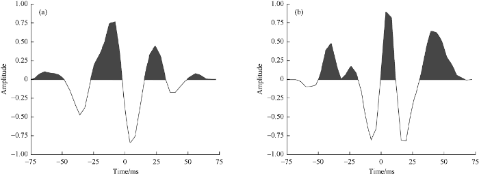
Fig. 1.
Wavelets extracted from 2D seismic sections.
In forward modeling, wavelet has a vital role in determining the amplitude, phase, and frequency of seismic data. The wavelets used in this study have proper amplitude and phase as they are from wire-line log and seismic data[64,65]. The amplitude spectrum was entirely obtained from statistics on seismic data, and the phase spectrum was extracted from the wire-line log data. The seismic wavelet extracted in this way ensures that the wellbore synthetic seismic trace is a good representative of near wellbore trace, and also the wellbore depth and seismic profile depth matched completely.
2. Results and discussions
2.1. Source of multifractality by MF-DFA
MF-DFA of original, surrogated and shuffled data can show the type and source of multifractality. Fig. 2 shows the dependency of H on q in the original, surrogated and shuffled series. When H>0.5, it shows positive correlation and persistent time series. The multifractality source of seismic trace has both long memory correlation and PDF broadness. The Hurst exponent difference between the shuffled and original series is greater than the Hurst exponent difference between the surrogated and original series. The multifractality caused by correlation is stronger than the multifractality caused by fat tail. This is because of two physical characteristics of formations: the depositional environment increases the correlation, while heterogeneity creates PDF broadness, they are both recorded by seismic data. The MF-DFA proved that these data have multifractality, and each layer has its own specific H value that represents its fractal characteristics.
Fig. 2.
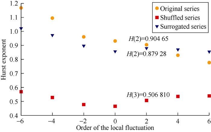
Fig. 2.
MF-DFA analysis results of original, surrogated and shuffled seismic traces.
2.2. Self-similar segmentation
In SAE model segmentation, the selected interval and variance of innovation e(t) are important. The Hurst exponent estimation is sensitive to the segment length of time series and the level of segmentation is affected by the variance of e(t). Both of them are examined and chosen by trial and error. Prior to execution of the final model, the model should be firstly tested to get the best time interval for evaluating Hurst exponent. Hurst exponent was estimated by several methods at different time intervals and identical results were found by comparing them. Secondly, after initializing the length of segments, the variance was engaged by the number of zones that the model was expected to find in the time interval. The ideal segmentation interval for the seismic traces was found to be 80 milliseconds. Smaller interval values would increase the error of Hurst exponent estimation and larger interval values decrease the resolution of segmentation. The optimum value for the variance of e(t) was chosen as 0.02. Larger values will decrease the number of zones and vice versa.
2.2.1. Theoretical wedge model analysis
Many studies have shown fractal properties of rocks are correlated with their characteristics in different scales. Rocks are good fractal bodies and their fractal features aren’t related to their scaling. These characteristics include rock type, total organic matter content, acid and reactive fluid contents in convection and diffusion processes, wettability, particle size, total pore volume, pore structure, sizes of intergranular and intragranular pores, specific surface area, clay mineral content, permeability, and so on. The results of these studies show that the estimated H depends on many factors. The H range for shale is between 0 and 1 and that for limestone is between 0.25 and 0. 65[66,67,68,69,70,71,72,73]. For synthetic wedge modeling, we analyzed two types of rocks, shale and limestone, and we assumed the average H values of limestone and shale were 0.45 and 0.7 respectively.
Wedge modeling is used to understand vertical resolution of some processing on seismic data. Tuning can make two reflected signals appear either as one signal or as no signal. Therefore, this thickness represents the minimum bed resolution that the wavelet can identify. In the current wedge modeling, we convolve Ricker wavelet with earth's reflectivity to work out the minimum resolution of SAE model. The average frequency of seismic data is 25 Hz, so a 25-Hz frequency Ricker wavelet was used for making a 2D zero-offset survey over a 20-degree wedge model. The surface layer is mudstone with a density of 2.3 g/cc and acoustic velocity of 3000 m/s, the wedge is limestone with a density of 2.6 g/cc and acoustic velocity of 5000 m/s. The wedge model has 2000 synthetic seismic traces that were recorded at a sample rate of 1 ms (field scale) and trace spacing of 1 m (field scale).
Reflectivity values of the wedge model are shown in Fig. 3a. SAE methodology uses fractal properties of the formations to detect and classify layers. Therefore, similar to real data, in shale region, the small reflection of fBm with H value of 0.7 is considered to be shale medium, and in the limestone wedge, the small reflection of fBm with H value of 0.45 is considered limestone medium. The reflection coefficient at the boundary of the two layers is about ±0.3, depending on acoustic impedance contrast of the two layers.
Fig. 3.

Fig. 3.
Reflectivity (a), seismic section (b), and SAE segmentation (d) of the wedge model (c).
The final 2D zero-offset profile of the wedge model is shown in Fig. 3b and its SAE segmentation for different traces is shown in Fig. 3c. It can be seen when the thickness of the wedge is smaller than 100 ms (thin bed), the model can only detect the first interface, CDP (common depth point) of 500, and when the wedge thickness is greater than 100 ms, both interfaces can be detected well (CDP of 1500 and 2000). When the wedge thickness is around 100 ms, the first interface is detected well, but the second interface is detected with error (CDP of 1000).
2.2.2. Field data analysis
The results of the SAE model segmentation on acoustic impedance logs, synthetic trace of A, B and C wells and the results of the SAE model segmentation on seismic traces around wells are shown in Figs. 4-6. To compare the curves better, x axes in all the plots were normalized between their minimum and maximum values.
Fig. 4.

Fig. 4.
Geological layering results by fractal method of seismic section crossing Well A.
Fig. 5.

Fig. 5.
Geologic layering results by fractal method of seismic section crossing Well B.
Fig. 6.

Fig. 6.
Geologic layering results by fractal method of seismic section crossing Well C.
As well A has part of acoustic impedance missing, so the layers of wells B and C were identified from acoustic impedance, synthetic traces, and seismic traces. In well B, tops of all layers were identified well on acoustic impedance and the seismic traces. Tops of six layers were identified clearly from the seismic traces, but F5 and F10 were identified with a little shift, and tops of layers F2, F4, and F9 weren’t identified. In well C, among tops of 8 layers, 6 of them were well identified by all kinds of data. Only the top of F1 wasn’t identified by acoustic impedance, and the top of F7 was only identified by acoustic impedance. In general, compared with log data, small layer thickness and low quality of seismic trace are two main reasons causing errors in identifying layers by SAE method.
In spite of the low quality of seismic data (with the highest resolution of about 10 meters), layers with specific fractal properties were identified accurately. In comparison, the wire-line logging data have a resolution of several inches, so the identification results with log data are litho-stratigraphic boundaries corresponding to lithological changes and are not always formation tops. Segmentation interval is another factor that can decrease the resolution of the results, because some recorded points are represented as new fractal points, the results of SAE model show small up and down shifts.
The results of self-similar segmentation on the acoustic impedance of wire-line log, synthetic and real seismic data were compared with the formation tops, it is found that in some cases the self-similar segmentation results of seismic data are more accurate in detecting formation tops. The results of this study are comparable with SAE model segmentation of wire-line log data by Shiri et al in 2012[2].
3. Conclusions
MF-DFA is an effective method to determine multifractal nature of signals like seismic data. By comparing the original, shuffled, and surrogated seismic traces, we found that the cause of multifractality is long-term correlation rather than PDF broadness in most cases. In addition, main factors affecting long term correlation and PDF broadness are depositional environment and heterogeneity. The SAE model segmentation proposed in this study was performed on post-stack seismic data and wire-line log data. The results prove that the SAE model segmentation of seismic data and wire-line log data can detect abrupt and transitional litological changes vertically. The SAE model segmentation based on intrinsic fractal properties of layers is an effective tool for identifying transitional and abrupt petrophysical variations in the earth layers. When the data available are seismic traces and conventional statistical methods can’t detect the earth layers, this method seems more effective.
Nomenclature
A(q,θ)—autoregressive part;
B(q,θ)—exogenous variable;
CDP—common depth point;
e(k)—a non-stationary white noise;
F(l,v)—variance of the detrended profile;
Fq(l)—local fluctuation;
h(q)—generalized Hurst exponent;
hshuffle(q)—generalized Hurst exponent of shuffled series;
H—Hurst exponent;
i—No. of a profile or time series;
j— summation within a part of the profile;
k—index of assumed variables and coefficients;
l—length of time series;
nb—last index of polynomial;
N—total number of time steps;
Nl—number of segments;
P(i)—profile;
Pv(i)—fitted polynomial;
q—order of the local fluctuation;
RXX(k)—auto-correlation of time series X;
S(ω)—power spectrum;
t—time;
T—transpose operator;
u(k), y(k)—signal;
X(t)— total travel time;
Xi—time series;
ŷ(k,θ)—a linear regression;
ξi—random variable that represents a step length;
τ—duration of time step;
ξN—length of time step;
ω—frequency;
θ—vector of coefficient;
φ(k)—part of the signal;
Reference
Sedimentology and petroleum geology: Book review
Self-affine and ARX-models zonation of well logging data
DOI:10.1016/j.physa.2012.05.025 URL [Cited within: 4]
Advances in geophysics
Correlation properties of (discrete) fractional Gaussian noise and fractional Brownian motion
Long-term storage capacity of reservoirs
Multifractal properties of pyrex and silicon surfaces blasted with sharp particles
DOI:10.1016/j.physa.2007.11.026 URL [Cited within: 1]
Self-affine gravity covariance model for the Bay of Bengal
DOI:10.1111/gji.2005.161.issue-1 URL [Cited within: 1]
Global and local multiscale analysis of magnetic susceptibility data
DOI:10.1007/s00024-003-2401-5
URL
[Cited within: 1]

Geophysical well-logs often show a complex behavior which seems to suggest a multifractal nature. Multifractals are highly intermittent signals, with distinct active bursts and passive regions which cannot be satisfactorily characterized in terms of just second-order statistics. They need a higher-order statistical analysis. In contrast with monofractals which have a homogeneous scaling, multifractals may include singularities of many types. Here we describe how a multiscale analysis can be used to describe the magnetic susceptibility data scaling properties for a deep well (KTB, Germany), down to about 9000 m. A multiscale analysis describes the local and global singular behavior of measures or distributions in a statistical fashion. The global analysis allows the estimation of the global repartition of the various Holder exponents. As such, it leads to the definition of a spectrum, D( ), called the singularity spectrum. The local analysis is related to the possibility of estimating the Lipschitz regularity locally, i.e., at each point of the support of a multifractal signal. The application of both approaches to the KTB magnetic susceptibility data shows a meaningful correlation between the sequence of Holder exponents vs. depth and the lithological units. The Holder exponents reach the highest values for gneiss units, intermediate ones for amphibolite units and the lowest values for variegated units. Faults are found to correspond to changes for H also when they are of intra-lithological type.
Measuring the fractal geometry of landscapes
DOI:10.1016/0096-3003(88)90099-9 URL [Cited within: 1]
Functional fractional calculus
Quantification of long-range persistence in geophysical time series: Conventional and benchmark-based improvement techniques
DOI:10.1007/s10712-012-9217-8
URL
[Cited within: 1]
Time series in the Earth Sciences are often characterized as self-affine long-range persistent, where the power spectral density, S, exhibits a power-law dependence on frequency, f, S(f) ~ f−β, with β the persistence strength. For modelling purposes, it is important to determine the strength of self-affine long-range persistence β as precisely as possible and to quantify the uncertainty of this estimate. After an extensive review and discussion of asymptotic and the more specific case of self-affine long-range persistence, we compare four common analysis techniques for quantifying self-affine long-range persistence: (a) rescaled range (R/S) analysis, (b) semivariogram analysis, (c) detrended fluctuation analysis, and (d) power spectral analysis. To evaluate these methods, we construct ensembles of synthetic self-affine noises and motions with different (1) time series lengths N = 64, 128, 256, …, 131,072, (2) modelled persistence strengths βmodel = −1.0, −0.8, −0.6, …, 4.0, and (3) one-point probability distributions (Gaussian, log-normal: coefficient of variation cv = 0.0 to 2.0, Levy: tail parameter a = 1.0 to 2.0) and evaluate the four techniques by statistically comparing their performance. Over 17,000 sets of parameters are produced, each characterizing a given process; for each process type, 100 realizations are created. The four techniques give the following results in terms of systematic error (bias = average performance test results for β over 100 realizations minus modelled β) and random error (standard deviation of measured β over 100 realizations): (1) Hurst rescaled range (R/S) analysis is not recommended to use due to large systematic errors. (2) Semivariogram analysis shows no systematic errors but large random errors for self-affine noises with 1.2 ≤ β ≤ 2.8. (3) Detrended fluctuation analysis is well suited for time series with thin-tailed probability distributions and for persistence strengths of β ≥ 0.0. (4) Spectral techniques perform the best of all four techniques: for self-affine noises with positive persistence (β ≥ 0.0) and symmetric one-point distributions, they have no systematic errors and, compared to the other three techniques, small random errors; for anti-persistent self-affine noises (β < 0.0) and asymmetric one-point probability distributions, spectral techniques have small systematic and random errors. For quantifying the strength of long-range persistence of a time series, benchmark-based improvements to the estimator predicated on the performance for self-affine noises with the same time series length and one-point probability distribution are proposed. This scheme adjusts for the systematic errors of the considered technique and results in realistic 95 % confidence intervals for the estimated strength of persistence. We finish this paper by quantifying long-range persistence (and corresponding uncertainties) of three geophysical time series—palaeotemperature, river discharge, and Auroral electrojet index—with the three representing three different types of probability distribution—Gaussian, log-normal, and Levy, respectively.
Intermittent turbulence in self-similar cascades: Divergence of high moments and dimension of the carrier
DOI:10.1017/S0022112074000711 URL [Cited within: 1]
Fractal theory and its implication for acquisition, processing and interpretation(API) of geophysical investigation: A review
DOI:10.1007/s12594-019-1142-8 URL [Cited within: 1]
Interpretation of gravity data using eigenimage with Indian case study: A SVD approach
DOI:10.1016/j.jappgeo.2013.05.004
URL
[Cited within: 1]
A new technique for delineation of subsurface features using gravity eigenimage is proposed to separate the gravitational anomalies from its background. The singular value decomposition and multifractal method has been combined and tested on several synthetic gravity anomalies and also applied to field gravity dataset of Vindhyan basin in central India which is a promising area for petroleum exploration. The eigenimage of gravity data helps to understand the relationship between the geological structure and source of anomaly. Fault structure is the major structure and could be the principal contributor that differentiates the regional and local geo-anomalies in the studied region. (c) 2013 Elsevier B.V.
Stock market efficiency: A comparative analysis of Islamic and conventional stock markets
DOI:10.1016/j.physa.2018.02.169 URL [Cited within: 2]
Scaling, multifractality, and long-range correlations in well log data of large-scale porous media
DOI:10.1016/j.physa.2011.01.010 URL [Cited within: 2]
A DFA approach in well-logs for the identification of facies associations
DOI:10.1016/j.physa.2013.07.052 URL [Cited within: 1]
Evolution of the temporal multifractal scaling properties of the Chiayi earthquake(ML=6.4), Taiwan
DOI:10.1016/j.tecto.2012.04.006 URL [Cited within: 1]
Power spectrum analysis and multifractal detrended fluctuation analysis of Earth’s gravity time series
DOI:10.1016/j.physa.2015.02.034 URL [Cited within: 1]
Reservoir characterization using multifractal detrended fluctuation analysis of geophysical well-log data
DOI:10.1016/j.physa.2015.10.103 URL [Cited within: 2]
Multifractal phenomena in physics and chemistry
DOI:10.1038/335405a0 URL [Cited within: 1]
Application of a time-scale local hurst exponent analysis to time series
DOI:10.1016/j.dsp.2014.11.007 URL [Cited within: 1]
Hybrid clustering-estimation for characterization of thin bed heterogeneous reservoirs
DOI:10.1007/s13146-018-0435-0 URL [Cited within: 1]
Flow and transport in porous media and fractured rock: From classical to modern approaches.
A survey of methods for time series change point detection
DOI:10.1007/s10115-016-0987-z
URL
PMID:28603327
[Cited within: 1]
Change points are abrupt variations in time series data. Such abrupt changes may represent transitions that occur between states. Detection of change points is useful in modelling and prediction of time series and is found in application areas such as medical condition monitoring, climate change detection, speech and image analysis, and human activity analysis. This survey article enumerates, categorizes, and compares many of the methods that have been proposed to detect change points in time series. The methods examined include both supervised and unsupervised algorithms that have been introduced and evaluated. We introduce several criteria to compare the algorithms. Finally, we present some grand challenges for the community to consider.
Seismic attributes for prospect identification and reservoir characterization
New seismic attribute: Fractal scaling exponent based on gray detrended fluctuation analysis
DOI:10.1007/s11770-015-0509-x
URL
[Cited within: 1]
Seismic attributes have been widely used in oil and gas exploration and development. However, owing to the complexity of seismic wave propagation in subsurface media, the limitations of the seismic data acquisition system, and noise interference, seismic attributes for seismic data interpretation have uncertainties. Especially, the antinoise ability of seismic attributes directly affects the reliability of seismic interpretations. Gray system theory is used in time series to minimize data randomness and increase data regularity. Detrended fluctuation analysis (DFA) can effectively reduce extrinsic data tendencies. In this study, by combining gray system theory and DFA, we propose a new method called gray detrended fluctuation analysis (GDFA) for calculating the fractal scaling exponent. We consider nonlinear time series generated by the Weierstrass function and add random noise to actual seismic data. Moreover, we discuss the antinoise ability of the fractal scaling exponent based on GDFA. The results suggest that the fractal scaling exponent calculated using the proposed method has good antinoise ability. We apply the proposed method to 3D poststack migration seismic data from southern China and compare fractal scaling exponents calculated using DFA and GDFA. The results suggest that the use of the GDFA-calculated fractal scaling exponent as a seismic attribute can match the known distribution of sedimentary facies.
Detection of seismic reflections from seismic attributes through fractal analysis
DOI:10.1046/j.1365-2478.2002.00323.x URL [Cited within: 1]
Correlation length and fractal dimension interpretation from seismic data using variograms and power spectra
DOI:10.1190/1.1487083 URL [Cited within: 1]
Development of oil development and gas prediction software system based on fractal dimension of amplitude spectrum
Detecting long-range correlations with detrended fluctuation analysis
DOI:10.1016/S0378-4371(01)00144-3 URL [Cited within: 1]
Effect of trends on detrended fluctuation analysis.
Effect of nonstationarities on detrended fluctuation analysis. Physical Review E: Statistical Physics, Plasmas, Fluids,
Scaling in nature: From DNA through heartbeats to weather
DOI:10.1016/S0378-4371(99)00340-4 URL [Cited within: 1]
Correlation approach to identify coding regions in DNA sequences
DOI:10.1016/S0006-3495(94)80455-2
URL
PMID:7919025
[Cited within: 1]
Recently, it was observed that noncoding regions of DNA sequences possess long-range power-law correlations, whereas coding regions typically display only short-range correlations. We develop an algorithm based on this finding that enables investigators to perform a statistical analysis on long DNA sequences to locate possible coding regions. The algorithm is particularly successful in predicting the location of lengthy coding regions. For example, for the complete genome of yeast chromosome III (315,344 nucleotides), at least 82% of the predictions correspond to putative coding regions; the algorithm correctly identified all coding regions larger than 3000 nucleotides, 92% of coding regions between 2000 and 3000 nucleotides long, and 79% of coding regions between 1000 and 2000 nucleotides. The predictive ability of this new algorithm supports the claim that there is a fundamental difference in the correlation property between coding and noncoding sequences. This algorithm, which is not species-dependent, can be implemented with other techniques for rapidly and accurately locating relatively long coding regions in genomic sequences.
Detection of changes in the fractal scaling of heart rate and speed in a marathon race
DOI:10.1016/j.physa.2009.05.029 URL [Cited within: 1]
Fractal properties of financial markets
DOI:10.1016/j.physa.2014.05.017 URL [Cited within: 1]
Music walk, fractal geometry in music
DOI:10.1016/j.physa.2007.02.079 URL [Cited within: 1]
Encyclopedia of complexity and systems science
Multifractal detrended analysis method and its application in financial markets
Multifractal properties of price fluctuations of stocks and commodities
DOI:10.1209/epl/i2003-00194-y URL [Cited within: 2]
Using surrogate data to detect nonlinearity in time series
Nonlinear dynamics time series analysis
Testing for nonlinearity in time series: The method of surrogate data
DOI:10.1016/0167-2789(92)90102-S URL [Cited within: 1]
Fractal and chaotic characteristics of seismic data
Research on the application of fractal and chaotic theory in exploration geophysics is just unfolding at present.However,perople still doubt whether seismic data have fractal and chaotic charcateristics.On the basis of power spectral analysis,we have derived the necessary conditions under which time series and seismic data will have fractal property.The power spectral analysis of real seismic data shows that seismic data satisfy fractal requirement within a certain frequency band,and that they also have chaotic characteristic.
Real-time prediction method of borehole stability
DOI:10.1016/S1876-3804(08)60012-9
URL
[Cited within: 1]
Abstract
Based on the close relationship between seismic and logging information, a real-time prediction model of borehole stability is established using seismic, logging, and geological data to control borehole wall sloughing instability. First, seismic attributes are extracted from borehole-side seismic traces of target wells and drilled offset wells. The mapping models of relationships between seismic attributes and logging data of various formation intervals in drilled wells are then constructed using wavelet neural network. Using the seismic attributes of formation under bit and the corresponding mapping model, the acoustic and density logging data of the current undrilled formation can be predicted. On the basis of the prediction results, the mechanical model of borehole stability is employed to calculate pore pressure, collapse pressure, and fracture pressure, thus predicting the safe drilling fluid density range. Practical application in Tarim Oilfield shows that real-time operation performance of the model is excellent and the prediction accuracy of parameters is satisfactory.
Autoregressive statistical pattern recognition algorithms for damage detection in civil structures
DOI:10.1016/j.ymssp.2012.02.014
URL
[Cited within: 1]
Statistical pattern recognition has recently emerged as a promising set of complementary methods to system identification for automatic structural damage assessment. Its essence is to use well-known concepts in statistics for boundary definition of different pattern classes, such as those for damaged and undamaged structures. In this paper, several statistical pattern recognition algorithms using autoregressive models, including statistical control charts and hypothesis testing, are reviewed as potentially competitive damage detection techniques. To enhance the performance of statistical methods, new feature extraction techniques using model spectra and residual autocorrelation, together with resampling-based threshold construction methods, are proposed. Subsequently, simulated acceleration data from a multi degree-of-freedom system is generated to test and compare the efficiency of the existing and proposed algorithms. Data from laboratory experiments conducted on a truss and a large-scale bridge slab model are then used to further validate the damage detection methods and demonstrate the superior performance of proposed algorithms. (C) 2012 Elsevier Ltd.
Wavelet and rescaled range approach for the Hurst coefficient for short and long time series
DOI:10.1016/j.cageo.2006.05.008
URL
[Cited within: 2]
Abstract
The calculation of Hurst coefficient (H) by different techniques is sensitive to the length of the profile and noise. Synthetic fractional Brownian motions with different values of H have been generated and the effectiveness of the techniques has been tested on these time series. H values are calculated by wavelet transform (WT), power spectrum (PS), roughness length (RL), semi-variogram (SV), and rescaled range (R/S) methods. On the basis of the error estimates two methods: R/S analysis and WT are suggested for calculation of H for short/long datasets. Further, WT method is applied to geophysical data of the Bay of Bengal. The gravity, magnetic and bathymetry data indicate the self-affine nature with H=0.8, 0.8 and 0.9, respectively.
A case study on discrete wavelet transform based Hurst exponent for epilepsy detection
DOI:10.1080/03091902.2017.1394390
URL
PMID:29188743
[Cited within: 1]
Epileptic seizures are manifestations of epilepsy. Careful analysis of EEG records can provide valuable insight and improved understanding of the mechanism causing epileptic disorders. The detection of epileptic form discharges in EEG is an important component in the diagnosis of epilepsy. As EEG signals are non-stationary, the conventional frequency and time domain analysis does not provide better accuracy. So, in this work an attempt has been made to provide an overview of the determination of epilepsy by implementation of Hurst exponent (HE)-based discrete wavelet transform techniques for feature extraction from EEG data sets obtained during ictal and pre ictal stages of affected person and finally classifying EEG signals using SVM and KNN Classifiers. The The highest accuracy of 99% is obtained using SVM.
Intelligent technologies and techniques for pervasive computing.
MATLAB system identification toolbox.
Segmentation of ARX- models using sum-of-norms regularization
DOI:10.1016/j.automatica.2010.03.013
URL
[Cited within: 1]
Abstract
Segmentation of time-varying systems and signals into models whose parameters are piecewise constant in time is an important and well studied problem. Here it is formulated as a least-squares problem with sum-of-norms regularization over the state parameter jumps, a generalization of ?1-regularization. A nice property of the suggested formulation is that it only has one tuning parameter, the regularization constant which is used to trade-off fit and the number of segments.
Detection of abrupt changes in signal processing.
System identification: Theory for the user. 2nd ed.
Initialization of output error identification algorithms
Crustal scale geometry of the Zagros fold- thrust belt, Iran
DOI:10.1016/j.jsg.2003.08.009
URL
[Cited within: 1]
Abstract
Balanced cross-sections across the Zagros fold–thrust belt in Iran are used to analyze the geometry of deformation within the sedimentary cover rocks, and to test the hypothesis of basement involved thrusting throughout the fold–thrust belt. Although the Zagros deformation front is a relatively rectilinear feature, the sinuous map-view morphology of the mountain front is a result of a 6 km structural step in the regional elevation of the Asmari Limestone that produces a pronounced step in topography termed the ‘mountain front flexure’. Although the height of the mountain front flexure is sufficient to permit basement fault–bend folds at the front of the Lorestan and Fars regions, the taper of the orogen, low percentage of shortening, and consistent structural elevation from the mountain front flexure to the hinterland suggest that Lorestan and Fars segments of the fold and thrust belt are completely detached on lower Cambrian salt and that basement-involved thrusting occurs only in the hinterland of the orogen. Mass balance constraints necessitate that detachment folds throughout the fold–thrust belt are cored by faults that branch from the basal detachment. The steep dips of these faults and their depth within the lower Paleozoic sedimentary rocks can account for recorded earthquakes. This suggests that the ∼11±4-km-deep earthquakes throughout the fold–thrust belt may be nucleating within sedimentary rocks rather than in the basement as previously proposed. Total shortening in the Zagros fold–thrust belt is 70±20 km, which corresponds to ∼20% shortening of the Arabian block.
Characterization and estimation of reservoir properties in a carbonate reservoir in Southern Iran by fractal methods
DOI:10.1007/s13202-017-0358-7 URL [Cited within: 1]
Comparison of wavelet estimation methods
DOI:10.1007/s12303-013-0008-0
URL
[Cited within: 1]
Wavelet estimation is a very important task in seismic data processing and analysis such as deterministic deconvolution, seismic-to-well tie, and seismic inversion, among others. We investigated the wavelets estimated from four different methods: (1) the wavelet estimated from the seafloor signal; (2) the wavelet estimated fully from well-log data; (3) the wavelet estimated using seismic and well-log data; and (4) the wavelet estimated from sparse-spike deconvolution. The wavelets estimated from 2-D seismic data using the four methods are quite comparable to one another. The results of the deconvolution and inversion of the 2-D seismic data using the four wavelets show that the wavelet estimated from the seafloor signal can be as effective as those estimated from the more rigorous methods.
A petroleum geologist’s guide to seismic reflection. New Jersey,
Fractal nature of acid-etched wormholes and the influence of acid type on wormholes
Two-scale (Darcy scale and pore scale) continuum wormholing models are built to study the fractal nature of the acid-etched wormholes in acidizing carbonate reservoirs and the influence of acid type on the conditions for wormholes to form. This model considers convection-diffusion mass transfer and reaction on the acid-rock interface, and the fractal dimension of dissolution patterns is calculated using box-counting method. The results show that wormholes are formed when convection and diffusion are equivalent in strength; when convection dominates, uniform dissolution is formed; when diffusion dominates, surface dissolution is generated. For the zones where the porosity is greater than 0.7, the fractal dimensions of the surface dissolution, wormholes and uniform dissolution are 1.46, 1.50 and 1.44, respectively, among which, the fractal dimension of the wormholes is approximate to the experimental results obtained by Daccord and Lenormand (1.6 +/- 0.1). The reaction between weak acid and rocks is controlled by reaction kinetics, the acid-etched wormholes are wide, and more acid is consumed. The reaction between strong acid and rocks is controlled by mass transfer, the acid-etched wormholes are narrow, and less acid is consumed. According to an example calculation, it is found that acidizing treatments should be performed in an isolated short section each time when the horizontal well is long.
Nano-scale pore structure and fractal dimension of lower Silurian Longmaxi Shale
DOI:10.1007/s10553-018-0933-8 URL [Cited within: 1]
Fractal analysis of shale pore structure of continental gas shale reservoir in the Ordos Basin, NW China
Nanopore structure and fractal characteristics of lacustrine shale: Implications for shale gas storage and production potential
DOI:10.3390/nano9030390 URL [Cited within: 1]
Full-scale pore structure and fractal dimension of the Longmaxi shale from the southern Sichuan Basin: Investigations using FE-SEM, gas adsorption and mercury intrusion porosimetry
DOI:10.3390/min9090543 URL [Cited within: 1]
Fractal measurements of sandstones, shales, and carbonates
The fractal properties of calcination of limestone and its sulfidation with H2S.
Fractal study on the complexity of limestone surface pore structure
DOI:10.4028/www.scientific.net/AMR.548 URL [Cited within: 1]
