Thin muddy interlayer has an important influence on oil sand steam assisted gravity drainage (SAGD), and it is also the main control factor of remaining oil distribution in the later stage of development. How to improve the prediction accuracy of muddy interlayer is an important problem in oil sand development. The thickness of muddy interlayer in oil sand reservoir is generally less than 20 cm, which is difficult to be identified by conventional logging curves, and its lateral extension prediction is more difficult. At the same time, the three-dimensional geological model of thin muddy interlayer often needs a number of tens of millions of grids, which brings a huge calculation burden to the reservoir numerical simulation. A coarsening process must be executed to reduce the number of grids to meet the needs of numerical simulation. However, thin muddy interlayer accounts for a small proportion of grids in the geological model, making it easily be filtered out by traditional coarsening methods, and the resulting model cannot reflect the influence of thin muddy interlayer.

Many scholars found that muddy interlayer has a great influence on the vertical permeability of reservoir and provided solution. Haldorsen et al. believed that the existence of muddy interlayer increases the tortuosity of streamline, thus reducing the vertical permeability, and then proposed the streamline method to calculate the effective vertical permeability of reservoir ^[1]. Based on this framework, Begg et al. expanded the streamline method from two-dimensional to three-dimensional, but this method is disadvantageous in that the whole geological model is regarded as one coarse grid^[2,3]. Green et al. provided the statistical function expression of the length and width of the muddy interlayer in 2D and 3D cases^[4], which is a statistical explanation to the vertical permeability coarsening equivalent calculation proposed by Begg et al. However, the tracking and statistics of the muddy interlayer in different coarsening grids within the reservoir range remain unresolved, impossibly supporting the actual reservoir production prediction. Li et al. achieved permeability characterization by calculating sandstone connectivity within the coarsening grid, and well reproduced the difference of per-meability values in different directions under the influence of muddy interlayer^[5]. However, Li’s method determines whether the grid value is effective by judging the sandstone connectivity across the whole coarsening grid, and uses the conventional weighted average for the effective permeability calculation in coarsening grid, without considering the increased fluid flow path caused by muddy interlayer. Thus, it exhibits a large error of permeability value in coarse grid.

This paper, based on the rich core data of Mackay River oil sand in Canada, carries out the prediction of muddy interlayer extension range, and puts forward the coarsening calculation method of permeability under the constraint of muddy interlayer, which reflects the influence of muddy interlayer on fluid flow to the maximum extent. Real reservoir simulations were executed and compared for verifying the effectiveness of the proposed method.

The Mackay River oil sand in Canada is located in Athabasca, Alberta, with an area of 760 km² and an estimated production capacity of 200 × 10⁴ t/a. The oil sand reservoir has the top buried depth of 160-180 m, the average net thickness of 18 m, the average saturation of 75%, the effective porosity of about 32%, and the permeability of 1-5 μm². There are 185 coring wells in the study area, with well spacing of 600-800 m.

According to the existing research results^[6,7,8,9], the Cretaceous McMurray Formation in the study area is divided into three sections, i.e. lower, middle and upper. The upper section (target section), affected by the tide and river actions, contains dominantly deposits of tidal sandbar and sand flat, with mixed flat deposits on both sides. In the weak hydrodynamic period, muddy drape deposits were developed, which are similar to the fall-siltseam of the mid-channel bar, and not completely preserved as a result of the tidal erosion. The core shows that the upper section is developed with muddy interlayer, with a few discontinuities, mostly horizontal and millimeter grade. The outcrop section shows that the muddy interlayer in the upper section is mostly horizontal, with poor continuity, and the extension distance mostly less than 10 m. The frequently developed muddy interlayers in the reservoir have very low permeability, and are even non-permeable, which directly hinders the existence of the steam cavity in the oil sand SAGD development and thus seriously affects the development effect.

Muddy interlayer has a serious impact on oil development^{[10,11,12,13,14]}. Its distribution scale can be predicted by using outcrop data^[15,16,17]. However, for some muddy interlayers that are only partially exposed, the statistics of the length obtained through outcrop observation is not complete. Geehan used the geometric probability to infer the length distribution of the muddy interlayer with unbiased property, under the premise of regularly square outcrop, which however is very difficult to find in field^[18]. White et al. put forward the use of termination frequency and Erlangian model to calculate the size of the muddy interlayer, which provides a new method for the prediction of the muddy interlayer^[19]. The method considers that the termination of the muddy interlayer on the outcrop is consistent with the actual situation of queuing time. The time interval between two people queuing, one waiting for the arrival of the other and waiting for the appearance of two people is equal to see the end of muddy interlayer on the outcrop section (the length of muddy interlayer can be measured within the outcrop range), seeing only one end of muddy interlayer and failing to see the end of muddy interlayer. The termination frequency is obtained by observing the occurrence of each end point of the muddy interlayer^[19]:

where n_T,i is the number of terminations of the i-th muddy interlayer observed on the finite outcrop exposure (n_T,i=0, 1 or 2). If the muddy interlayer completely crosses the outcrop area, the number of terminations is 0. If one end extends out of the outcrop area, the number of terminations is 1. If neither end extends out of the outcrop area, the number of terminations is 2.

The probability of 0, 1 or 2 terminations observed can be calculated by geometric probability respectively:

For the muddy interlayer with length l, the average number of terminations observed is:

By substituting Formulas (3) and (4) into Formula (5), we can get the expected number of terminations:

According to Formula (6), if l is far less than λ, two ends are expected; if l is far greater than λ, no end is observed; if l is equal to λ, one end is always observed.

On the outcrop section with a length λ, the probability that a muddy interlayer with a length l can be observed is:

The expected average number of terminations of the muddy interlayer with a length l can be calculated by the following formula:

As observed, the average length of the muddy interlayer with different numbers of ends is:

Then, the formula (9) is rewritten as:

Besides, the expected length of the muddy interlayer with different numbers of ends is:

By substituting formulas (8) and (11) into formula (1), we can obtain a simplified calculation formula of termination frequency:

and the calculation formula of the average length of the muddy interlayer:

As along as the number of ends of the muddy interlayer in the core is counted, the termination frequency of the muddy interlayer can be determined, and then formula (13) is used to calculate the average extension length, so that the scale of the muddy interlayer is predicted.

2.2.1. Statistics of termination frequency and prediction of scale of muddy interlayer in cores

The 185 coring wells in the Mackay River oil sand reservoir basically cover the whole area. The continuity of muddy interlayer in core can be considered equivalent to the sampling observation of muddy interlayer distribution in subsurface reservoir. The extension length of the muddy interlayer can be predicted according to the termination of the muddy interlayer on the core photo.

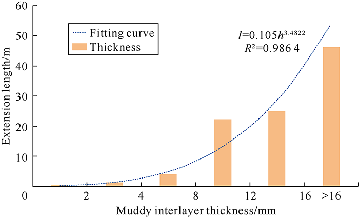
According to the statistics of 50 coring wells in the study area, 5905 muddy interlayers were identified, including 5544 through the whole core barrel, in other words, 5544 muddy interlayers have 0 end, with a probability of 93.9%, 253 muddy interlayers have 1 end, with the probability of 4.3%, and 108 muddy interlayers have 2 ends, with the probability of 1.8%. Specifically, the muddy interlayers with 2 ends have the average length of about 40 mm, and the average thickness of about 2 mm. The average length calculated based on the termination frequency is 0.1 m, which is quite comparable with the above-mentioned average length 0.04 m. Based on the termination frequency, the average length is calculated to be 1.19 m for the 2-4 mm thick muddy interlayers, 3.86 m for the 4-8 mm thick muddy interlayers, which is close to the average extension length of 0.87 m observed on outcrop, and 45.92 m for the thick muddy interlayers larger than 16 mm (Table 1).

The predicted extension range of the muddy interlayer using the termination frequency is also comparable with the actual interpretation results. Burton et al. observed and interpreted the outcrop of Sego sandstone in Utah, indicating that the length of completely terminated muddy interlayer is 0.1- 15.0 m, with an average of 5.0 m, and the length of muddy interlayer predicted by the termination frequency is 0-45.0 m, with an average of 16.3 m^[20]. In this paper, the distribution of the inclined muddy interlayers in the McMurray Formation is also predicted. The fine anatomy of the reservoir structure shows that the extension length of the inclined muddy interlayers is 37.2-107.0 m, and the average extension length of the muddy interlayers predicted by the proposed method in this paper is 67.8 m. The longer extension of the inclined muddy interlayer is mainly attributed to the good continuity of the inclined muddy interlayer. Thus, the termination frequency derived from core observation can be used to predict the extension length of the muddy interlayer.

Regression analysis was carried out between the statistical thickness of muddy interlayer and the calculated extension length, showing a significant positive correlation (Fig. 1). The lateral scale of the muddy interlayer can be characterized by the thickness of the muddy interlayer obtained from the well data.

2.2.2. Three-dimensional geological modeling of muddy interlayer

Since muddy interlayer is approximately horizontal, with large distribution frequency and short extension, its shape can be simplified as a cuboid, and its three-dimensional distribution can be predicted by the method of marked point process modeling. The marked point process is a common stochastic geological modeling method^{[21,22,23,24,25,26,27]}. Spatial points are generated by point distribution function, and then the object attributes (e.g. object type, geometric shape, etc.) are given at this point. When the target attribute percentage reaches the specified threshold, no space points are generated and a simulation result is obtained. The sandstones in the study area are widely and continuously distributed with thin muddy interlayers. The background facies can be set as sandstone facies, and then thin muddy interlayers are simulated in the sandstone background. The simulated termination condition is controlled by the percentage of muddy interlayers counted by wells.

When establishing the model, different sampling values of length and width are given according to the thickness of muddy interlayer. For example, when the thickness of muddy interlayer is 8-12 mm, the uniform distribution function is selected, the lower limit is 8 mm, the upper limit is 12 mm, and the average value is 10 mm. The muddy interlayer thickness of the grid point is randomly sampled, and the muddy interlayer extension length is determined by the relationship between the thickness and length of the muddy interlayer established in Fig. 1. According to the scale of muddy interlayer, the size of simulation grid is set to 5 m× 5 m × 2 mm, and the total number of grids is 343 × 231 × 2100 = 166389300. The relevant parameters are set up, and the marked point process modeling is used to achieve the three-dimensional spatial distribution prediction of the muddy interlayer (Fig. 2). The established model well reproduces the shape and spatial distribution of muddy interlayers with different thicknesses. On the whole, the muddy interlayers are nearly horizontal, small in scale and high in development frequency. Most of the muddy interlayers only pass through one well, and a large number of muddy interlayers are randomly distributed between wells.

The permeability model adopts sequential Gauss simulation method, with well-interpreted permeability value as reference, and the muddy interlayer is set as non-permeable, so the permeability model is established (Fig. 3). The overall permeability value of the model is high, generally more than 500 × 10^{- 3} μm². At the same time, there are a large number of local low- permeability areas of muddy interlayer under this background.

The existence of muddy interlayer will change the fluid flow path and affect the distribution of remaining oil. In essence, such change is manifested in increasing the flow length of fluid through the space, which is equivalent to the flow tortuosity in microstructure. Therefore, the coarse grid is regarded as the macrostructure, while the internal muddy interlayer is the microstructure. The permeability in different directions can be calculated by the Darcy formula only by determining the tortuous path of the flow tube under the constraint of the muddy interlayer^[1,2,3].

Apply the Darcy's law to each flow tube:

In the vertical direction, the total flow is:

Substituting ${Q_j}$ into Formula (15):

Assuming that each flow tube has the same cross-sectional area,

So,

Substituting Formula (18) into Formula (16), then

Obviously, once the tortuosity of each flow tube is determined, the mean value of the equivalent permeability affected by the muddy interlayer vertically can be calculated by formula (19). Based on statistical theory, Green et al. gave the calculation formula of average flow path length^[4]

If there are enough randomly distributed muddy interlayers in the reservoir, the number of muddy interlayers encountered by each flow tube is relatively constant. In three-dimensional case, the average value of the shortest flow path is:

When the width of the muddy interlayer is larger than the length of the muddy interlayer, only the positions of $\bar w$ and $\bar l$ need to be interchanged. If S_j is replaced by β, formula (19) can be simplified as:

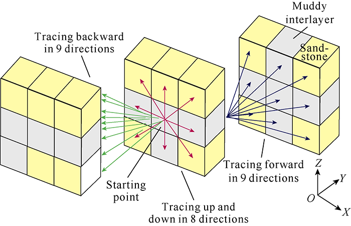
It can be seen that the difficulty in calculating the flow path length is to obtain the average length and width of the muddy interlayer in the coarse grid. Deutsch et al. designed a method to trace sandstone body and calculate connected sandstone volume in coarse grid^[28]. The core of the method is to take each coarse grid as a model, which contains several fine grids; one of the fine grids is selected, and muddy interlayer points are tracked along the adjacent grids of the one selected (Fig. 4). In the three-dimensional case, for each grid, adjacent grids in 26 directions will be tracked to obtain the connectivity range of muddy interlayers. Using this method, the three-dimensional body of muddy interlayers can be obtained. In this paper, the three-dimensional body is projected on the XOY, YOZ and ZOX planes, respectively, so that the projection area of the muddy interlayer in Z direction, X direction and Y direction can be obtained. On the XOY plane, the extension length or width of the muddy interlayer is obtained grid by grid in the X or Y direction. Then the average length and width of the muddy interlayer in the Z direction can be obtained, and the equivalent coarsening of the muddy interlayer calculated based on the tortuous path can be realized.

A fine geological model comprises a huge number of grids, making it infeasible to be directly applied to reservoir numerical simulation. Generally, it needs to be coarsened, namely, the model with tens of millions of grids is equivalent to one with millions of or hundreds of thousands of grids. Because the muddy interlayer is thin, it is often filtered out by traditional coarsening method, so that its influence on the development of steam cavity and reservoir development effect cannot be reflected. Therefore, it is necessary to find a new coarsening method to retain the characteristics of the muddy interlayer to the maximum extent and meet the demand of fine numerical simulation.

The equivalent coarsening method based on tortuous path proposed in this paper and the equivalent coarsening method based on flow behaviors commonly used in commercial software are used to coarsen the fine model to grids of 113 × 75 × 25 = 211875. In Fig. 5, the coarsening model based on tortuous path exhibits an area with the permeability of 0, because the interlayer completely passes through the whole coarse grid, which can reflect the shielding effect of the muddy interlayer on the fluid. In Fig. 6, the coarsening model based on flow behaviors can hardly reveal the shielding effect of muddy interlayer, because there is no area with the permeability of 0, but the permeability only decreases significantly in local area.

It can be seen in Fig. 7 that, compared with the fine geological model, the equivalent coarsening model based on tor-tuous path contains less muddy interlayers, but reserves the obvious shielding effect of muddy interlayers in local area; the equivalent coarsening model based on flow behaviors does not reflect the shielding effect of the muddy interlayers, which only significantly reduce the permeability but do not hinder the flow of fluid. Clearly, the equivalent coarsening method based on tortuous path is more accurate.

A local area (grid size 50 × 50 × 25) in the coarsening model is selected for verification. With the original fine geological model, the equivalent coarsening model based on tortuous path and the equivalent coarsening model based on flow behaviors, the SAGD reservoir numerical simulation is carried out.

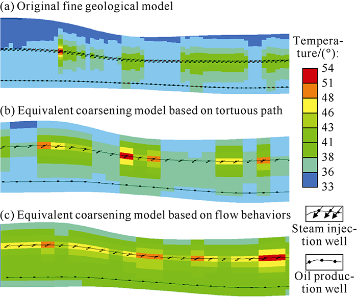
As shown in Fig. 8, the results of the equivalent coarsening model based on tortuous path are similar to those of the original fine geological model, both of which exhibit that, in local area, due to the muddy interlayers with low (or 0) permeability, steam cannot spread effectively, the temperature is low, the expansion of steam cavity is limited, and the distribution of temperature field is uneven. In contrast, the equivalent coarsening model based on flow behaviors shows extensive spread of steam, relatively even distribution of temperature field, and the smooth expansion of steam cavity. Essentially, the shielding effect of muddy interlayer is filtered out in the process of equivalent coarsening based on flow behaviors, and the permeability field is relatively smooth after coarsening.

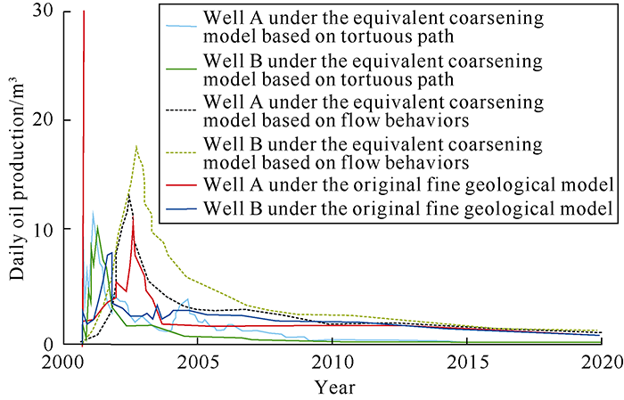
In Fig. 9, for the equivalent coarsening model based on flow behaviors, which does not consider the shielding effect of muddy interlayer on flow, the daily oil productions of Well A and Well B are the highest, and they are close to those for the original fine geological model at the initial stage but much higher at the middle and later stages. For the equivalent coarsening model based on tortuous path, the daily oil productions of Well A and Well B are close to those for the original fine geological model at the initial stage, with similar peaks of oil production, but lower than those for the original fine geological model at the middle and later stages. The production in the simulated calculation is lower because a part of crude oil is not included after coarsening. Such part of crude oil remains in the coarse grid and has migrated laterally and been produced, although the permeability of the muddy interlayer completely passing through the grid is set to 0, making it an empty grid, and the very thin muddy interlayer only takes an extremely small proportion of the grid.

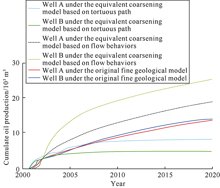
Similar rules can be observed from cumulative oil production. In Fig. 10, the equivalent coarsening model based on flow behaviors shows the highest cumulative oil productions of Well A and Well B, followed by the original fine geological model, and the equivalent coarsening model based on tortuous path shows the lowest cumulative oil productions. On the whole, the equivalent coarsening method based on tortuous path considers the shielding effect of muddy interlayer, and its numerical simulation results are closer to those of the fine geological model, and can more effectively represent the impact of the actual geological conditions. Therefore, the equivalent coarsening method based on tortuous path is effective.

Application in the west area of Long Lake Field, Canada has proved that the equivalent coarsening model based on tortuous path effectively reflects the influence of the tide-dominated meandering river point bar lateral accretion layer on the development effect and shows a good fitting performance. Therefore, the proposed method can be applied to equivalent coarsening of different types and occurrences of muddy interlayers.

The muddy interlayers in the Mackay River oil sand cores are 2-12 mm thick, with the termination frequency of 0.04- 19.64 and the extension length of 0.10-45.92 m. The thickness has a good positive correlation with the extension length, which can be used to establish a quantitative function to predict the three-dimensional distribution of muddy interlayer.

The comparisons of coarsening results and development indexes prove that the equivalent coarsening method based on tortuous path can well reflect the shielding effect of the muddy interlayer, and can more effectively represent the impact of actual geological conditions on the development effect. The proposed method is effective and practical.

$\bar d$—intermediate variable, m;

F_s—percentage of muddy interlayer, %;

H—reservoir thickness, m;

h—muddy interlayer thickness, m;

i—muddy interlayer number;

j—flow tube number;

k—muddy interlayer end number;

K—reservoir permeability, 10^-3 μm²;

K_VE—reservoir vertical permeability, 10^-3 μm²;

l—length of muddy interlayer, m;

l_i—length of the i-th muddy interlayer, m;

$\bar l$—average length of muddy interlayers;

$\tilde l\left( {l,\lambda } \right)$—average length of muddy interlayers with the length of 0-l observed on the outcrop with a length of λ, m;

$\bar \tilde l\left( {\lambda ,{\chi _l}} \right)$—the expected average length of muddy interlayers with the length of 0-l observed on the outcrop with a length of λ, m;

L—reservoir length, m;

m—number of muddy interlayer on outcrop;

n_T—number of muddy interlayer terminations;

${\tilde n_{\rm{T}}}\left( {l,\lambda } \right)$—average number of terminations observed of muddy interlayers with length of l on the outcrop with a length of λ;

${\bar \tilde n_{\rm{T}}}$—the expected average number of terminations observed of muddy interlayers;

N_s—number of flow tubes;

$p\left( {{n_{\rm{T}}} = k\left| {l,\lambda } \right.} \right)$—probability of the k-th termination of muddy interlayer, k = 0, 1, 2;

$p\left( l \right)$—development probability of muddy interlayer with the length of l, dimensionless;

$\tilde p\left( {l\left| \lambda \right.} \right)$—probability that the muddy interlayer with the length of l is observed on the outcrop with the length of λ, dimensionless;

Q_j —flow rate of j-th flow tube, mm²/s;

Q_T —flow rate of fluid, mm²/s;

${r_1}$ and ${r_2}$—stochastic value sampled form the uniform distribution over (0~1), dimensionless;

S_j—length of the j-th flow tube, m;

$\hat t$—average termination frequency of the muddy interlayer on the outcrop, determinations/m;

W_j —streamline width of the j-th flow tube, m;

w_i —width of the i-th muddy interlayer, m;

$\bar w$—average width of muddy interlayers, m;

β—average path of the flow tube under the influence of the muddy interlayer, m;

$\Delta p$— pressure difference at both ends of the flow tube, MPa;

λ—outcrop length, m;

μ—fluid viscosity, mPa·s;

τ—development frequency of muddy interlayers, interlayers/m;

χ_l—average length of muddy interlayers with the length of 0-l, m.