Introduction
A reliable prediction of well construction time is an important element in the planning of oil and gas exploration and development[1]. To predict and optimize drilling time, most attentions have been paid to model the rate of penetration (ROP). Traditional ROP models[2,3,4,5,6,7,8] have been developed, incorporating major variables to represent the drilling processes. They are referred to as semi-empirical models, in which physical variables are combined with multiple regression to formulate the predictive equation. In recent years, the establishment of modern ROP models, which take advantage of complex drilling data and assessable computational resources, is growingly popular[9]. Such models are mainly data-driven, solvable by the application of various statistical and machine learning techniques, such as artificial neural networks (ANN)[10,11,12], random forest[11,13], and support vector machines[13].
While ROP modelling provides an important measure to assess the efficiency of drilling, it is just a component of the total well construction time. Previous studies[14-15] pointed out that the improvement in both instantaneous and averaged ROPs does not necessarily lower the cost of drilling. This is because a drilling operation consists of several operational phases, from mobilizing the drilling unit, pulling out bottom hole assembly (BHA) for changing worn-out bits, casing and cementing, resolving incidental issues, many of which are unable to be directly attributed to ROP. The total well construction time can also be affected by non-productive factors, such as failure of a drilling equipment, longer than expected “fishing time” for lost objects, or stormy weather. The non-productive time during an entire drilling operation could last multiple days, which is of the same order as the productive time spent on the mechanical drilling of wellbore alone. Therefore, modelling the complete well construction time is critical for a better planning of drilling operations.
The modelling of the well construction time can be derived by either the deterministic approach or the probabilistic one. In the deterministic approach, the drilling time is an expected value obtained from a model, which is established from its relationships with all drilling elements. Multiple regression analysis had been applied for the entire well construction time[16,17,18], or for a phase of drilling such as the duration to exchange the drill bits[19,20]. Recent progress in this approach has been empowered by the machine learning techniques. For example, Ardekani et al.[19] developed an ANN model for the mechanical duration for replacing drill bits, which is shown to be more accurate than the regression for sampling southern Iranian oil fields. The probabilistic approach considers the estimated time as a likelihood rather than a single number. It is based on the fact that the occurrence of events during a drilling course is not deterministic, regardless of the most careful planning process, but instead is a stochastic process driven by a wide range of non-deterministic factors. The probabilistic approach allows the operators to not only understand comprehensively the uncertainties of drilling activities, but also quantify the risks for better optimization of drilling costs[21,22]. These facts explained why this approach became a common business practice in well construction industry during the last two decades[23,24]. McIntosh[21] presented a probabilistic analysis for durations of individual drilling phases based on sample data and suggested that ranking such probabilities will be helpful in prioritizing the activities that have higher impact on their overall objective. Akins et al.[22] established a relatively comprehensive set of management practices for adopting the probabilistic approach for forecasting well construction time. Loberg et al.[23] and Merlo et al.[24] further completed commercial software packages that allow drilling engineers to quantify the risks and translate them into corresponding values of duration and cost. Using the database of 118 wells in the central North Sea, Adams et al.[25] characterized the probability distributions of the drilling duration classified by a wide range of factors. In 2015, Adams et al.[26] updated the progress with finer probability distributions by adding 93 new wells into consideration. Despite having a noticeable success, one major limitation of these probabilistic models is that they are based solely on the univariate probability density function (PDF). Some bias occurred because the multivariate PDF was oversimplified to the univariate case by ignoring the higher dimensions such as vertical length and depth of drilling.
This study proposes to apply the multivariate PDF to characterize and predict the well construction time. First, we are able to incorporate more drilling variables into the probabilistic modelling and thus improve the accuracy of the overall prediction. Second, we can obtain the conditional probability after certain events have occurred, and hence can better quantify the predictability. We focus on the predictability of total durations of major mechanical drilling phases, including conductor hole, surface hole, intermediate hole and construction hole, since the majority of the drilling time is spent on them. In our multivariate analysis, we adopt the target depth for modelling drilling phases, and the vertical distance for modelling casing and cementing phases. A preliminary analysis indicates that these depth-dependent measures have highest correlation with the required times in each phase.
In this study, our proposed models of time for each phase are based on the self-consistent kernel density estimation, and models of time for an entire operation are combined using Markov chain Monte Carlo simulations. To demonstrate the feasibility of our multivariate approach, we carried out a case study using observed data from 192 wells. We first present probabilistic models for the trouble-free time. We then present the validation of our models, discuss the difference between total time versus trouble-free time, and explore the possibility of the model output to generate data for training of machine learning models.
1. Multivariate probabilistic approach
First, we utilize the self-consistent kernel density estimation technique to obtain the multivariable probabilistic density function of different well construction phases. Based on this, we estimated the distributions of well construction time that take into account the drilling depth and other various parameters. We employed the Monte-Carlo simulations to combine probabilities of different well construction phases to form prediction models for complete drilling operation.
1.1. Multivariate probabilistic density functions (PDF)
The multivariate PDF is formed by the joint occurrences of two or more variables. In this study, we use the self-consistent kernel density estimation method developed by Bernacchia and Pigolotti[27] to derive the multivariate PDF. Its advantage is the capability to derive an optimal and objective selection of both the kernel and the bandwidth (bin) with excellent convergence property. We adopt the implementation of O'Brien et al.[28], namely fastKDE, which produced a fast and efficient estimation of the PDF for a large amount of data.
Let us consider the multivariate probability density function f on a data set that has n data points p1, p2, …, pn. Here, our kernel density estimation (KDE) is two-dimensional, consisting of the well construction time t and the depth-dependent variable d, which is the other parameter that depends on individual phases. Each element of dataset pj can be represented by the coordinate (tj,dj) for j=1, 2, …, n. Note that we can add more variables into the KDE to represent the distribution in higher dimensions. Our probability density function $\hat{f}$ is a function of smooth variable p, whose relationship with the discrete data points p1, p2, …, pn is established via the involvement of a kernel function K:
Obviously, in order to obtain the probability density function $\hat{f}$ from a set of discrete data points, we have to determine the form of kernel function K. The self-consistent KDE method introduced by Bernacchia and Pigolotti[27] involves the application of the Fourier transform, an efficient technique to convert the data coordinate (t,d) into the frequency domain u that describes the distribution and vice-versa. Here, the inverse Fourier transform is defined as
The Fourier transform of optimal kernel function is given by
The key to the self-consistent KDE method is that the optimal estimate $\hat{\kappa }(u)$ of function $\kappa (u)$ can be associated directly with the optimal inverse $\hat{\phi }(u)$
where E(u) is an empirical characteristic function to be defined as
The substitution of $\hat{\phi }(u)$ from Equation (4) in Equation (3) helps deriving the explicit optimal value $\hat{K }(u)$ [27]:
The main process to obtain the PDF $\hat{f}(p)$ from the set of input data can be summarized as follows: ① Construct the empirical characteristic function E(u) from the set of input data p1, p2, …, pn as per Equation (5). ② Deduce the optimal estimate $\hat{\kappa }(u)$ from Equation (6). ③ Derive the form of $\hat{\phi }(u)$ from Equation (4). ④ Obtain the probability density function $\hat{f}(p)$ after the Fourier transform as per Equation (7).
1.2. Markov chain Monte Carlo simulations
The predictability of each phase of drilling can be derived from the PDF. However, it is difficult to achieve a confident predictability of entire drilling operations when a lot of data are missing. Suppose that we want to estimate the time of a complete operation that consists of all major phases. While there are only 2% of operations consisting of all phases, we may have to ignore precious information from the majority of data (98%). When the number of complete operations is not large enough, the predictability will be biased due to the small samples used.
Fortunately, the Markov chain Monte Carlo (MCMC) method allows us to take advantage of the PDF that we obtained from individual phases to generate sampling data, and thus conveniently and effectively estimate the risks associated with the entire operation. The use of MCMC in estimating the uncertainties of drilling operation is not new[29]. Peterson et al.[30] successfully applied to simulate the risks of the Authorized for Expenditures (AFE). However, the results were not robust since they used a small number of data (27 wells) and assumed that the inputs belong to a number of special distributions: Normal, Gamma, Lognormal and Exponential.
In this study, we adopted the Gibbs sampler, an MCMC algorithm to generate a sequence of data from a multivariate PDF. Although the Gibbs sampler is a special case of the well-known Metropolis-Hastings (MH) sampler, it performs better in multi-dimensions because the generalization of MH algorithm makes it sensitive to the choice of jumping function. The process to generate r simulations of a drilling operation that consists of m phases using the Gibbs sampler is summarized as follows:
Step 1. Start the process with initial samples $p_{1}^{k}(t_{1}^{k},d_{1}^{k})$ from the distribution $\hat{f}({{t}^{k}},{{d}^{k}})$ of the individual phase k for k=1, 2, …, m.
Step 2. Assume we have i samples $p_{1}^{k},p_{2}^{k},...,p_{i}^{k}$ in the phase k, and we want to generate the next sample, that is $p_{i+1}^{k}$, and add it into the list. From the latest sample $p_{i}^{k}(t_{i}^{k},d_{i}^{k})$, we randomly select the depth $d_{i+1}^{k}$ from the conditional probability $\hat{f}({{d}^{k}}\left| t_{i}^{k} \right.)$ to have the intermediate (temporal) value $p_{i}^{*k}(t_{i}^{k},d_{i\text{+}1}^{k})$. After that, we randomly select the time $t_{i\text{+}1}^{k}$ from the conditional probability $\hat{f}({{t}^{k}}\left| d_{i+1}^{k} \right.)$. Then we have the entire new sample $p_{i\text{+}1}^{k}(t_{i\text{+}1}^{k},d_{i\text{+}1}^{k})$ to be added into the list.
Step 3. Repeat Step 2 for all k from 1 to m, so that we have a MCMC simulation that consists of m phases.
Step 4. Repeat (Step 2 and Step 3) r-1 times, so that we have a total number of r Monte Carlo simulations ($p_{1}^{k},p_{2}^{k},...,p_{n}^{k}$ for k=1, 2, …, m)
The process is the same for the dimensions higher than two. It is noted that in such case, the order of variables in Step 2 is randomly selected for each step of getting the sampling from conditional distributions.
2. Descriptive analysis of a case study
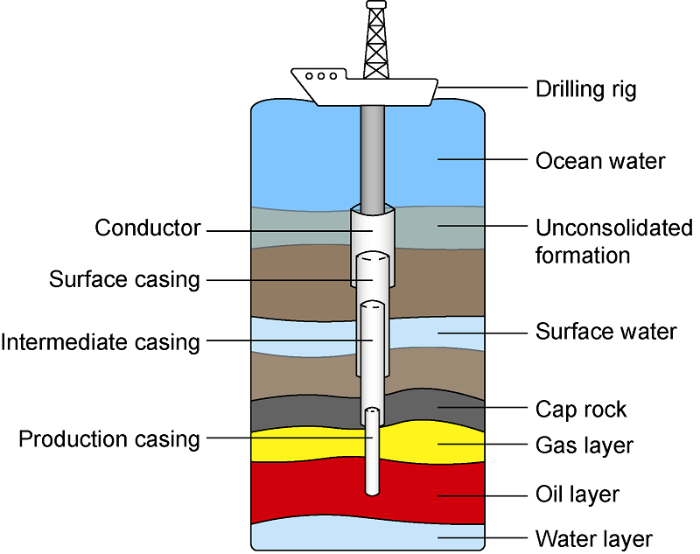
Our industry partner is a company in Malaysia who provides data management services for multiple drilling companies. We use a dataset that has 192 operations in the database (Table 1). Each operation data consists of the sequence of phases in an operation, duration of each phase and the depth information. Fig. 1 depicts the major phases of a typical successful well drilling operation. As we focus on a set of 8 major phases associated with the drilling, other phases are discarded from the dataset. In the rest of this section, we discuss these 8 major phases, which can be clustered into 4 groups as follows.
Table 1 Summary of 414 operations in the drilling database with respect to different category classification.
| Category | Classification | Total number | Used wells | Percentage of used wells/% | Percentage of used wells by category/% |
|---|---|---|---|---|---|
| Well type | Development | 152 | 68 | 45 | 35 |
| Exploration | 66 | 53 | 80 | 28 | |
| Production | 191 | 69 | 36 | 36 | |
| Others | 5 | 2 | 40 | 1 | |
| Drilling type | Offshore | 410 | 192 | 47 | 100 |
| Onshore | 4 | 0 | 0 | 0 | |
| Region | Australia | 380 | 176 | 46 | 92 |
| Asia | 26 | 13 | 50 | 7 | |
| Unknown | 8 | 3 | 38 | 1 | |
| Rig type | Semi-submersible | 127 | 100 | 79 | 52 |
| Drillship | 28 | 20 | 71 | 10 | |
| Others | 14 | 0 | 0 | 0 | |
| Unfilled | 245 | 72 | 29 | 38 | |
| Spud year | 1996 | 4 | 0 | 0 | 0 |
| 2006 | 7 | 7 | 100 | 4 | |
| 2007 | 30 | 23 | 77 | 12 | |
| 2008 | 42 | 22 | 52 | 11 | |
| 2009 | 35 | 16 | 46 | 8 | |
| 2010 | 34 | 21 | 62 | 11 | |
| 2011 | 34 | 15 | 44 | 8 | |
| 2012 | 30 | 17 | 57 | 9 | |
| 2013 | 15 | 3 | 20 | 2 | |
| 2014 | 22 | 7 | 32 | 4 | |
| 2015 | 39 | 11 | 28 | 6 | |
| 2016 | 29 | 10 | 34 | 5 | |
| 2017 | 29 | 18 | 62 | 9 | |
| 2018 | 52 | 20 | 38 | 10 | |
| 2019 | 12 | 2 | 17 | 1 |
Fig. 1.
Fig. 1.
Major phases of a typical successful well drilling operation.
2.1. Drilling conductor hole (CH) and conductor casing (CC)
The main purpose of the conductor or conductor hole (CH) is to establish a functional stability of the well, wellhead and operating equipment by providing a solid structural base during the initial drilling activities. When the drilling starts, the conduit will carry the drilling muds from the borehole back to the rig. The preparation process for the conductor hole often takes 0.35 days (about 8.4 hours), as observed from the dataset (Table 2). The follow-up phase is conductor casing (CC), which consists of a pipe hammered into the seabed with cements using a pile driver. The pipe is very thick (>3 cm) and short, while having a large diameter of size 47-51 cm, putting inside the hole of size 61-66 cm[31]. On average, the casing is completed in about 0.78 days (about 18.7 hours) (Table 2). The correlation between the casing time of conductor hole (CC) and the depth change is as small as 0.18, probably due to the fact that there is no actual vertical drilling being triggered yet.
Table 2 Statistics of phases of interest available in 192 selected operations in the dataset.
| Phase | Number of record | Duration/days | ||||||
|---|---|---|---|---|---|---|---|---|
| Minimum | Maximum | Mean | Median | Variance | Skewness | Kurtosis | ||
| CH | 49 | 0.02 | 0.86 | 0.35 | 0.31 | 0.04 | 0.54 | -0.27 |
| SH | 132 | 0.02 | 13.83 | 1.87 | 1.28 | 4.23 | 2.88 | 11.00 |
| IH | 130 | 0.01 | 21.17 | 5.18 | 4.29 | 16.94 | 1.41 | 2.14 |
| PH | 132 | 0.01 | 15.31 | 3.68 | 3.43 | 6.59 | 1.19 | 2.71 |
| CC | 112 | 0.01 | 3.06 | 0.78 | 0.77 | 0.27 | 1.11 | 2.62 |
| SC | 132 | 0.05 | 4.65 | 1.55 | 1.39 | 0.70 | 0.90 | 1.18 |
| IC | 104 | 0.02 | 11.08 | 2.38 | 2.16 | 2.46 | 2.09 | 8.44 |
| PC | 23 | 0.08 | 5.42 | 1.81 | 1.65 | 1.78 | 0.99 | 0.77 |
2.2. Drilling surface hole (SH) and surface casing (SC)
The phase after the completion of conductor casing is the drilling of surface hole (SH). It is designated to ground the drilling activities from the surface toward the deeper layer, which are commonly suffered from the weak geological formation and the penetration of fresh waters into the wellbore. It takes 1.9 days on average (Table 2) for drilling a hole of an approximate diameter of 45 cm. Sometimes, it may take up to nearly 14 days for this phase to be fully finished. After that, the following up casing phase is to start deploying strings of case, aiming at isolating the movements of fluids and equipment within the wellbore and the surrounding environment. The typical casing diameter is a bit smaller, about 34 cm, allowing for the fulfilment of cements. The mean duration for casing phase is 1.55 days on average (Table 2). The Pearson’s correlation between drilling time and depth change is as high as 0.80, indicating that we can estimate the corresponding duration required for drilling to a target depth.
2.3. Drilling intermediate hole (IH) and intermediate casing (IC)
The longest phase in an operation is the drilling of intermediate hole (IH). It takes an average of 5.2 days to complete drilling the hole within this phase (Table 2). It is of great challenge to model precisely the durations of IH phase due to the fact that various sophisticated factors influence the time, from geological characteristics of the seabed, properties of the wellbore, types and handling of equipment as well as various unexpected technical and non-technical incidents occurred that may delay the process. This fact is supported by the large variance as shown in our dataset (Table 2). Once the hole is ready, its casing phase (IC) only takes 2.4 days to complete (Table 2). The typical diameters of the surface hole and its casing are 31 cm and 24 cm, respectively[31].
2.4. Drilling production hole (PH) and production casing (PC)
A production hole (PH) drilling is required to reach the target depth of oil reservoir, which often takes 3.7 days (Table 2). More technical issues arise in preparing this final hole, which explains why the longest operation may be up to 2 weeks. A production casing (PC) is installed from the rig to the target depth to seal off the production zones, providing the ground for extraction of oil. The production hole and case typically have diameters of 22 cm and 18 cm, respectively. The mean duration for casing phase is 1.8 days on average (Table 2). Due to cost and technical issues, the production casing may be occasionally replaced by a production liner in deep wells.
3. Probabilistic model system of trouble-free well construction time
In order to establish the probabilistic model system of trouble-free well construction time, we made two assumptions that are commonly adopted in practice in reconstructing the PDF as well as carrying out the MCMC simulations. First, we assume that the number of data points observed is in a good and complete representativeness of actual distribution of a drilling phase. Second, we assume that duration of each phase is a stochastic process which contains inherent randomness in both the inputs and outputs, and each phase has an independent random process that is not correlated to each other.
3.1. Depth-dependent probabilistic models of individual phases
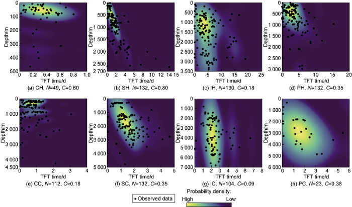
We are able to establish the joint probability distributions of well construction time and depth, estimated from the self-consistent Bernacchia-Pigolotti kernel density estimation method[27] for different phases: Conductor hole drilling (CH), Surface hole drilling (SH), Intermediate hole drilling (IH), Production hole drilling (PH), Conductor hole casing (CC), Surface hole casing (SC), Intermediate hole casing (IC) and Production hole casing (PC) as shown in Fig. 2. Some characteristics of these phases presented in Fig. 2 can be summarized as follows. First, the well construction times of all phases are the superpositions of multiple ellipsoid regions. Each ellipse is a region where the distribution of points is denser toward its centre. Second, most of the phases, namely SH, IH, PH, CC, SC and IC, have their major axes of main ellipses not uniformly or parallelly elongated in the horizontal direction but inclined toward the increasing depth. Third, the inclinations of ellipses of CH, SH, PH, SC and PC phases (yellow and green shades in Fig. 2a, Fig. 2b, Fig. 2d, Fig. 2f and Fig. 2h) coincide with the directions of diagonal lines in the phases that have high Pearson’s correlation coefficients (in the range of 0.35-0.80) between time and depths. The distributions in Fig. 2 allow us to obtain a conditional probability for predicting the time from a given depth or vice-versa (that is, obtaining the depth from a given time).
Fig. 2.
Fig. 2.
Joint probability distributions of TFT time and depth for 8 different phases.
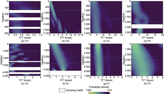
We first focus on the predictability of trouble-free time. Fig. 3 represents the spatial distribution of conditional probability of the trouble-free time with respect to the given depths for different phases. Horizontal lines denote the distance where we extract the sample one-dimensional conditional probability of well construction time with respect to that given distance (which will be used later in Fig. 4). Fig. 3 shows that the likelihood of the well construction time is not the same value, but it is actually varied proportionally to their variations. This result aligns with our intuition that the deeper the borehole is, the longer it takes to drill or implement the casing and cementing to the target depth.
Fig. 3.
Fig. 3.
Spatial distribution of conditional probability of the TFT time with respect to the given depths for 8 different phases. The horizontal white bands show the regions of low probability, that are cut off after the Fourier transform.
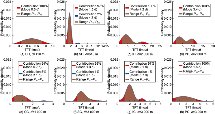
Given the conditional probability, we can obtain the predicted time for individual phase at a given depth. Fig. 4 represents conditional probability distribution of the trouble-free time associated with a given sampling distance. For example, the conditional probability to drill for a vertical distance of 2000 meters in the Drilling Intermediate Hole (IH) phase is depicted in Fig. 4c. Overall, Fig. 4 shows larger values in the vertical axis, indicating a higher probability of obtaining the drilling time, where the PDF is decomposed into multiple dominant modes. The PDF curve and the contribution of each mode (in percentage) are depicted in the figures, excluding the PDF curves with contribution percentage less than 1% or beyond plot windows. In the example of IC phase (Fig. 4g), the probability is peaked at 2.1 days in the first dominant mode (accounted for 97% of the chance) and at 6.7 days for the second dominant mode (accounted for 1% of the chance). It indicates that the trouble-free time is 2.1 days with the highest chance and 6.7 days with the second highest chance. Brown shaded regions in Fig. 4 are to represent the P10-P90 range of each mode. Having IC phase as the example (Fig. 4g), the P10-P90 range of trouble-free time for the first mode is between 1.1 to 3.8 days.
Fig. 4.
Fig. 4.
Conditional probability distribution of the TFT time with respect to a given depth for 8 different phases.
In summary, these probabilistic models allow us to predict the time to complete a certain drilling or casing phase for a given vertical distance. We provide estimation of the dominant modes, showing its highest chance for occurrence within the range. The result is given in the probabilistic range with minimum and maximum, allowing the operators to quantitively estimate the risk in the drilling plan instead of a deterministic point estimate that does not reflect the nature of unpredictability in the actual drilling.
3.2. Monte Carlo-based model of a complete operation with trouble-free time
One of the greatest challenges we have to deal with is inadequate data. In our dataset, there are only 2% of the operations having all 8 phases, and most of the operations have only 3-5 phases. In addition, all phase data are either over leptokurtic (kurtosis>3) or platykurtic (kurtosis <3) (Table 2), posing a challenge in applying regular point-based statistical models. This difficulty is further compounded by the fact that the data histogram is positively skewed out of normal distribution. As the data of these eight phases are not available at all operations, it is difficult to simultaneously consider all of them at the same time in a single model.
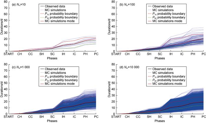
Using Monte-Carlo simulations, we are able to derive the likelihood of a complete operation that consists of all 8 phases for the trouble-free time as exhibited in Fig. 5. In Fig. 5, Markov chain Monte Carlo simulations for the TFT time for different number of experiments are presented for a complete operation by blue lines. The solid black lines are the observed data, which are derived from arithmetic means of original data for each phase. It is found that when the number of simulations is 1000 or above, the ensemble average of all operations generated from Monte-Carlo simulations is about 20 days (Fig. 5c and Fig. 5d, red lines), which is almost the same as the average time of original phases from observational data as of 19 days (Fig. 5c and Fig. 5d, blue lines). In other words, our MCMC experiments are able to capture well the deterministic mean of original data. The P10-P90 percentile range is stable after 1000 experiments, estimated to be 15-29 days. In some cases, the duration of a complete operation can last up to 43 days, a risk that is non-excludable. Note that while Fig. 5 demonstrates the results for the random walk from all values of phases
Fig. 5.
Fig. 5.
Markov chain Monte Carlo simulations for the TFT time for different number of experiments (N).
in the given available range of depth of each phase, we can also determine the MCMC results for a fixed depth.
In summary, Monte Carlo simulations allow us to estimate the well construction time based on a large number of simulations. The advantage of this method is that it does not require the simultaneous availability of data in all phases as a complete operation. Instead, we can combine the operations that may contain missing data in a complete risk assessment. The larger number of simulations is, the better quantification we are able to achieve for the risk in the entire drilling operation.
4. Discussions
4.1. Model validations
The establishment of statistical or probabilistic models from given datasets is often regarded as sufficient for its use in practice in many cases without any supplementary evaluation[32,33,34]. However, in this study, we further carry out an extra analysis to validate the models because of two reasons. First, it is necessary to compare and verify the optimality of parameters obtained in our models. Second, it is useful to match the modelled parameters against the actual drilling parameters in order to understand whether our models are able to capture the main features of data. The validation become more and more important as we need to deal with the issue of data inadequacy in establishing our models.
One of the challenges in reconstructing the PDF is the subjectiveness of the optimal choice of parameters, including the prior form of function and bin (or bandwidth). The KDE method is subjective to the selection of both kernel bandwidth and kernel shape. By applying the Fourier transform on the empirical characteristic function, Bernacchia and Pigolotti[27] showed that a low-pass filter can help deriving a self-consistent KDE that optimally minimizes the difference between the modelled PDF and the actual one. The self-consistent KDE is proved to be fully convergent when the number of samples is large, and it is not influenced by the subjective choice of kernel bandwidth and kernel shape.
The cut-off frequency is the only parameter that is required in establishing the self-consistent KDE, which Bernacchia and Pigolotti[27] suggested to be such that a half of the empirical characteristic function values is above a certain empirical threshold. O'Brien et al.[28] extended the KDE by incorporating the Fast-Fourier Transform (FFT) and come up with an alternative empirical threshold associated with the set of so-called hypervolumes. Bernacchia and Pigolotti[27] demonstrated that their threshold works efficiently with artificial data, whilst O'Brien et al.[28] showed that their parameter is efficient and stable for both artificial data and the realistic case of climate data. Moreover, O'Brien et al.[28] also proved that their choice of optimal parameter performed as excellent as other automatic bandwidth selection methods. For that reason, we adopted the O'Brien et al.’s method[28] and their default empirical threshold.
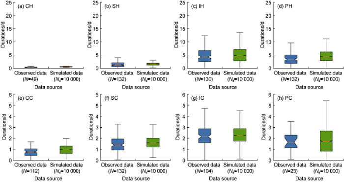
Fig. 6 presents a statistical comparison between the observed data and the data generated from our multivariate models for different phases. For the observed data, we tally all points that are available in each phase. For the modelled data, we adopted 10000 points that are generated from the probabilistic model for each phase eliminating abnormal points. It is found that the statistics of modelled data and the observed data are highly similar. For example, the median of modelled parameter of the Drilling Intermediate Hole (IH) phase (Fig. 6c) is 4.9 days, which is closely matched with the observed median of 4.3 days (Table 2).
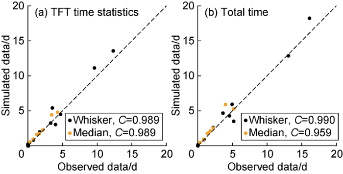
To fully examine the performance of our models, we have summarized the medians and whiskers of statistical boxplot parameters for all phases in Fig. 6. The summarization of these parameters for the trouble-free time is presented in Fig. 7a. It is found that the medians and whiskers of the phases in our models have an excellently high correlation with the observed data, with the Pearson’s correlation coefficients as high as 0.989. In the total time (Fig. 7b), the results are the same with the high correlation coefficients as of 0.990 and 0.959, respectively. It is noteworthy to mention that the number of data points available in each phase is about only 132 or lesser. Despite this difficulty, the modelled parameters are perfectly matched with the actual drilling parameters.
Fig. 6.
Fig. 6.
Statistical comparison between the observed data and the data generated from our multivariate probabilistic models for 8 different phases.
Fig. 7.
Fig. 7.
Comparison of statistical parameters between the observed data and the data generated from our multivariate probabilistic models.
4.2. Difference between trouble-free and total time
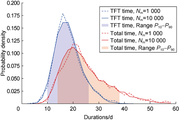
There is always a significant difference between the trouble-free time and the total time. To quantify the difference, we repeated the process to derive the depth-dependent probabilistic models of individual phases for total time. Then we carried out the new MCMC experiments for the total time for all operations in the dataset. Fig. 8 shows the probabilistic distribution for trouble-free time and total time with MCMC experiments. For trouble-free time, The P10 and P90 values of TFT are 10 and 26 days, respectively. In other words, 80% of probability for drilling a complete operation will be a time in between 10 days and 26 days. In comparison, the P10 and P90 values of total time is 14 and 38 days, respectively. It implies that the problem occurs during drilling is likely to delay the time by at least 4 days, and at most 12 days. Furthermore, the shape of the total time PDF is elongated along the horizontal axis with a longer tail, implying that not only the duration is longer but also uncertainty range is larger.
Fig. 8.
Fig. 8.
Probability distribution of a complete operation MCMC simulations for TFT time and total time.
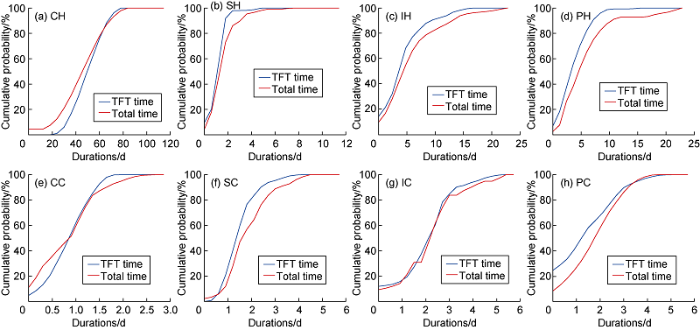
Fig. 9 depicts the cumulative probability distribution function for trouble-free time and total time of each phase after 10000 MCMC simulations. It is found that production hole drilling (PH) has the most significant difference between the trouble-free time and total time, which is occasionally larger than 10 days (at cumulative probability as of 95%). Drilling surface (SH) and intermediate (IH) holes could occasionally last longer than 2 days (at cumulative probability as of 95%).
Fig. 9.
Fig. 9.
Cumulative probability distribution of each phase after 10000 MCMC simulations for TFT time and total time.
4.3. Application in generating drilling data
An interesting application of probabilistic approach is that it allows us to generate the data from the probability distribution function. It is significant because machine learning models relied on the availability of data. Data inadequacy has been known to cause degradation in performance of such models. To further examine the possibility of probabilistic approach in improving the predictability of machine learning models, we tested the performance of a random forest (RF) model against different numbers of input data.
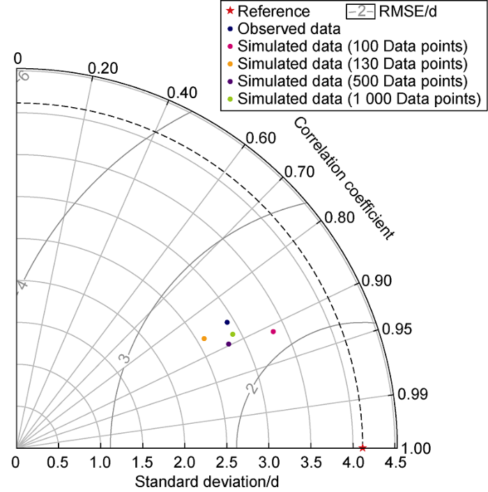
Fig. 10 depicts the performance of RF model against a wide range of numbers of input data using the Taylor diagram. The diagram allows us to compactly assess all three key statistics in a single figure, namely the Pearson’s correlation coefficient, the root-mean-square error (RMSE), and the standard deviation. It is found that all generated data have similar standard deviation as of the original data, with a range from 2.5 to 3.3 days. At the same time, the RMSE is in the range of 2.2 to 2.6 days. Especially, the RF performs well in all cases, with the Pearson’s correlation coefficients being very high (>0.8). It indicates that the generated data has similar features with the original ones. In other words, our models can be adopted to generate drilling data for better training of machine learning algorithms.
Fig. 10.
Fig. 10.
Comparative performance of Random Forest model with different numbers of input data.
5. Conclusions
We presented an approach to predict the well construction time with multivariate probabilistic models. The success of the work is attributed to the application of self-consistent kernel density estimation technique to construct depth-dependent probabilistic models of well construction time and the harnessing a combination of density distributions by means of Markov chain Monte-Carlo simulations for a complete drilling operation including all phases. We tested our model using a dataset provided by our industry partner. The data in the dataset are collected during the actual drilling operation of the wells. The results show that our models can be used to derive the likelihood of durations of each of the 8 major operation phases at a certain depth and the combined them for an entire drilling operation. We also found that problem occurs during the drilling operation is very likely to delay the time by at least 4 days, and at most 12 days. Last but not least, the data generated from the probabilistic approach can be used for a better training of machine learning models.
Nomenclature
C—Pearson’s correlation coefficient;
d—depth, m;
E(u)—empirical characteristic function;
f—multivariate probabilistic density function;
$hot{f}$—optimal f;
F—Fourier transform;
F-1—reverse Fourier transform;
i—Sample SN;
j—point SN;
k—drilling phase SN;
K—kernel;
m—number of phases;
n—number of points;
N—number of drilling phases with data record available, number of records in short;
Nd—number of points used for statistics of simulations;
Nm—number of MC experiments;
p—smooth variable;
p1, p2, …, pn—discrete data points;
P10, P90—Probabilities for confidence level of 10% and 90%, respectively, %;
r—number of MC simulations which consists of all drilling phases;
t—well construction time, d;
u—frequency domain;
κ(u)—Fourier transform of kernel density function;
$\hat{K}(u)$—optimal κ(u);
ϕ(u)—inverse Fourier transform;
$\hat{\phi}(u)$—optimal inverse transform.
Reference
Harness oil and gas big data with analytics
The “perfect-cleaning” theory of rotary drilling
DOI:10.2118/408-PA URL [Cited within: 1]
A new approach to interpreting rock drill ability
Microbit studies of the effect of fluid properties and hydraulics
DOI:10.2118/1520-PA URL [Cited within: 1]
A multiple regression approach to optimal drilling and abnormal pressure detection
DOI:10.2118/4238-PA URL [Cited within: 1]
Roller-bit penetration rate response as a function of rock properties and well depth.
Estimating the drilling rate in Ahvaz oil field
DOI:10.1007/s13202-013-0060-3 URL [Cited within: 1]
Drilling rate of penetration prediction and optimization using response surface methodology and bat algorithm
Real-time prediction of rate of penetration during drilling operation in oil and gas wells.
Use of machine learning and data analytics to increase drilling efficiency for nearby wells
DOI:10.1016/j.jngse.2017.02.019 URL [Cited within: 1]
A comprehensive data mining approach to estimate the rate of penetration: Application of neural network, rule based models and feature ranking
DOI:10.1016/j.petrol.2017.06.039 URL [Cited within: 2]
Drilling data from an enhanced geothermal project and its pre-processing for ROP forecasting improvement
DOI:10.1016/j.geothermics.2017.12.007 URL [Cited within: 1]
Petroleum well drilling monitoring through cutting image analysis and artificial intelligence techniques
DOI:10.1016/j.engappai.2010.04.002 URL [Cited within: 2]
Drilling efficiency and rate of penetration: Definitions, influencing factors, relationships and values
Efficient drilling time optimization with differential evolution
Drilling time predictions from statistical analysis
A mathematical model for analysing drilling performance & estimating well times
Systems for automated drilling AFE cost estimating and tracking
Development of drilling trip time model for southern Iranian oil fields: Using artificial neural networks and multiple linear regression approaches
DOI:10.1007/s13202-013-0065-y URL [Cited within: 2]
Development of a trip time for bit exchange simulator for drilling time estimation
DOI:10.1016/j.geothermics.2017.07.006 URL [Cited within: 1]
Probabilistic modeling for well-construction performance
Enhancing drilling risk and performance management through the use of probabilistic time & cost estimating.
The how’s and why’s of probabilistic well cost estimation.
An innovative tool on a probabilistic approach related to the well construction costs and times estimation.
Probabilistic well-time estimation revisited.
Probabilistic well-time estimation revisited: Five years on.
Self-consistent method for density estimation.
DOI:10.1111/rssb.2011.73.issue-3 URL [Cited within: 8]
A fast and objective multidimensional kernel density estimation method: FastKDE
DOI:10.1016/j.csda.2016.02.014 URL [Cited within: 6]
Monte Carlo techniques applied to well forecasting: Some pitfalls
Brief: Risk analysis and Monte Carlo simulation applied to the generation of drilling AFE estimates
DOI:10.2118/30887-JPT URL [Cited within: 1]
Oilwell drilling engineering: Principles and practice
Sea level trend and variability in the Singapore Strait
DOI:10.5194/os-9-293-2013 URL [Cited within: 1]
Sea level trend and variability around Peninsular Malaysia
DOI:10.5194/os-11-617-2015 URL [Cited within: 1]
Global mean sea level rise during the recent warming hiatus from satellite- based data


