Multilateral wells promise cost savings to oil and fields as they have the potential to reduce overall drilling distances and minimize the number of slots required for the surface facility managing the well. However, drilling a multilateral well does not always increase the flow rate when compared to two single-horizontal wells due to competition in production inside the mother-bore. Here, a holistic approach is proposed to find the optimum balance between single and multilateral wells in an offshore oil development. In so doing, the integrated approach finds the highest Net Present Value (NPV) configuration of the field considering drilling, subsurface, production and financial analysis. The model employs stochastic perturbation and Markov Chain Monte-Carlo methods to solve the global maximising-NPV problem. In addition, a combination of Mixed-Integer Linear Programming (MILP), an improved Dijkstra algorithm and a Levenberg-Marquardt optimiser is proposed to solve the rate allocation problem. With the outcome from this analysis, the model suggests the optimum development including number of multilateral and single horizontal wells that would result in the highest NPV. The results demonstrate the potential for modelling to find the optimal use of petroleum facilities and to assist with planning and decision making.
Keywords:multilateral well;
horizontal well;
well pattern optimisation;
drilling cost;
Net Present Value;
offshore oil development
ALMEDALLAH Mohammed, ALTAHEINI Suleiman Khalid, CLARK Stuart, WALSH Stuart. Combined stochastic and discrete simulation to optimise the economics of mixed single-horizontal and multilateral well offshore oil developments. PETROLEUM EXPLORATION AND DEVELOPMENT, 2021, 48(5): 1183-1197 doi:10.1016/S1876-3804(21)60101-5
Introduction
Multilateral wells have been employed extensively in petroleum operations since the 1980s due to their higher production rates and superior reservoir contact than single wells. They are also favored due to their lower drilling costs and reduced requirements for offshore platform slots[1,2,3,4,5,6]. However, the production of a multilateral well is not always equal to the production sum of the same single horizontal wells drilled separately as the branches of the multilateral well[7]. Particularly when multiphase flow is present, reduced performance can result due to interference and commingled outflow at the intersection point of the parent wellbore[7,8]. These factors can offset the benefits of lower drilling and facility costs that come with drilling a multilateral well. A multi-disciplinary team is required to evaluate a multilateral development once a candidate reservoir is selected[9,10]. The team conducts separate studies that optimize the wellbore trajectory, reservoir management strategy, production, surface facility and economics to assist in the decision making. While optimization studies that combine two or more of these efforts in a single model have advanced our understanding of multilateral developments[11,12], they fall short for field development planning because they overlook either drilling, facility, reservoir or economical perspectives. Several drawbacks may result from not including one of these aspects in the optimization. For instance, optimizing the production inside the wellbore without studying the impact on the surface facilities leads to an overestimated or underestimated production rates[8]. Likewise, the optimal number of multilateral wells cannot be determined without information about the capacity of the wellhead platform[13]. To overcome this limitation, this paper outlines an integrated mathematical model for maximizing the NPV of multilateral well developments. In particular, it investigates the optimum balance between the saving in drilling costs and potential production loses to suggest the optimal economic mix of single and multilateral wells while analyzing the surface facility, drilling trajectory, reservoir productivity as well as the economics of the field.
A number of prior studies have compared the productivity of vertical, horizontal, and multilateral wells by analyzing one or more key field development problems. Joshi[14], Retnanto et al.[15], Salas et al.[7] and Furui et al.[16] focused on finding a representation for the inflow relationship but ignored other critical field development problems such as the well path and surface facility integration. Yeten[12] expanded the previous work by not only studying the inflow relationship but also optimizing the well type, location and trajectory of multilateral wells using Genetic Algorithms and Artificial Neural Networks. His trajectory optimization represented each lateral and main-bore with straight lines, ignoring the curved sections of a realistic path. Lian et al.[17] studied the effects of the outflow. They used Greens Functions and Newman’s product to describe the reservoir inflow and wellbore outflow. Studies by Longbottom[18], Stalder et al.[19], Yaliz et al.[20] and Cetkovic et al.[21] cover notable examples of field applications of multilateral developments. However, these studies lack the integration required to simultaneously conduct the lateral path optimization with the pipeline and facility allocation. To overcome these limitations, here an integrated approach is proposed that honors the physical interactions of reservoir, wellbore trajectory, pressure network and facility infrastructure. Implementing this integrated model has several benefits, including (but not limited to) minimizing planning time, providing a more accurate production forecast, and hence better economic analysis to support decision making.
1. Model description
We consider a shallow-water offshore field with multiple reservoirs that contain several well targets (WT) that must be drilled to boost production. Each target is defined by two points: a target entry (TE) which is the starting point of the reservoir section and a target depth (TD) describing the end point of the same section. The infrastructure required to drill and produce these targets include: a wellbore, a wellhead, a wellhead platform (WP), a tie-in platform (TP) and a separation and processing facility (SPF). The wellbore is used to transport the fluid from the target to the wellhead and can be drilled as a single horizontal well or a multilateral well. An example of this infrastructure connectivity is shown in Fig. 1.
Fig. 1.
A multilateral development highlighting the main infrastructure required to drill the targets.
The model’s objective is to maximize the development NPV over a predetermined planning horizon by evaluating potential single-horizontal and multilateral well configuration. The input data includes the field or lease boundary, the onshore location of separation processing facility (SPF) and its inlet pressure, the location of well targets, basic reservoir, tubing and pipeline properties, a phase behavior model and economic data assumptions such as discount rate. From these input data, the model determines the surface facility output, including the number, location, water depth, size of all surface facilities, number of pipelines and their route and connectivity. It also generates the drilling configuration which is described in terms of the number of single-horizontal wells or multilateral wells and their three dimensional wellbore trajectory. The model not only selects between single-horizontal or multilateral developments but it also suggests the optimum economic mix of these development options. In addition, the model calculates a reservoir pressure decline, production portfolio for each well and the dynamic pressure and flow rates of each node in the system. The model also imposes real-world drilling and production facility constraints on the design of the field. The drilling constraints include the maximum number of laterals per well, maximum measured allowable depth and dog-leg severity based on available rig’s limitation. It also accounts for facility constraints such as the maximum wells per wellhead platform; the maximum wellhead platforms per tie-in platform; the minimum water depth to install the wellhead and tie-in platforms; as well as the maximum distance between any two wellhead or tie-in platforms. We assume that all reservoirs are undersaturated, i.e. the reservoir pressure is above the bubble point. However, as the fluid enters the wellbore and surface pipelines, the pressure in these components may fall below the bubble point, causing outgassing and two-phase flow. This is an active problem to deal with in an oil field. Therefore, in this work, the model employs the K-means clustering method developed by Macqueen to assist with setting up the initial solution for the problem instead of having a complete random initial solution[24]. For the subset initial solution such as lateral allocation problems where a gradient-free algorithm would be costly to use, a Mixed Integer Linear Programming (MILP) is chosen to provide an initial estimate. Then, a global optimization method involving a stochastic perturbation coupled with Markov Chain Monte-Carlo (MCMC) is presented to solve for the global field plan. Once a configuration has been found, an estimate of its productivity is required to calculate the Net Present Value. The user can connect the optimization algorithm to one of the existing commercial software that estimates production flow rates and pressure parameters for a field configuration. However, in this model, we have developed our own production flow simulator to improve the interface between the resulting field configuration and productivity estimation.
In summary, the optimization routine employed in this analysis consists of the following stages:
1. An initial solution for the field is established using K- means clustering developed by Macqueen[14] and Mixed-Integer Linear Programming (MILP) technique for a full-single-horizontal development.
2. Next, the optimum wellbore trajectory for all possible lateral and single-horizontal wells in the field is found according to dogleg severity and drilling reach using a gradient-free linear approximation technique known as COBYLA [25].
3. A new MILP algorithm is then applied to optimize the lateral to single-horizontal connectivity based on maximum laterals per well and maximum wells per wellhead platform.
4. The pipeline network and route are then optimized using a global method involving a combined Dijkstra algorithm as developed by Dijkstra [26] and COBYLA optimization to find the pipe path.
5. Next, the reservoir, wellbore and surface network productivity is calculated using a Levenberg Marquardt Deterministic optimization technique as explained by Lourakis [27].
6. The future dynamic performance of the reservoir is ac- counted for by using material balance such that an initial NPV for the project is calculated.
7. To improve the global solution, the system is perturbed using stochastic perturbation combined with MCMC. Steps 2 to 6 are then repeated to find a better field configuration.
1.1. Initial solution
Here, the problem is initialized by assuming that the field consists entirely of single-horizontal wells (i.e. no multilateral wells are initially included). Instead of generating a random number, size and position of surface facilities to drill these targets, a combined K-means clustering and Mixed-Integer Linear Programming (MILP) are introduced to provide this initial solution. Using K-Means[24], we can cluster groups of well targets in our input data which are closer to one another and allocate them to the same wellhead platform and assign an initial position for wellhead platform to be the center of this group of wells.
Once an initial position is estimated for all NWP wellhead platforms, the location of all possible lateral- branching point is determined which will have the same horizontal coordinates of the WP, while the vertical depth is chosen by the user. In this model, the user can specify a single depth or provide a range of formation depths where branching can start. After determining these branch points, all possible well paths that can drill each well target are calculated and their cost is determined from$\sum\limits_{{{i}_{\text{wt}}}=1}^{{{N}_{\text{wt}}}}{\sum\limits_{{{i}_{\text{b}}}=1}^{{{N}_{\text{b}}}}{{{C}_{\text{l},{{i}_{\text{wt}}},{{i}_{\text{b}}}}}{{\Lambda }_{\text{l,}{{i}_{\text{wt}}},{{i}_{\text{b}}}}}}}$. Alternatively, the well paths may also consist of single-horizontal wells without any branch-ing. The cost of these single-horizontal wells is repre-sented by$\sum\limits_{{{i}_{\text{wt}}}=1}^{{{N}_{\text{wt}}}}{\sum\limits_{{{i}_{\text{wp}}}=1}^{{{N}_{\text{wp}}}}{{{C}_{\text{s},{{i}_{\text{wt}}},{{i}_{\text{wp}}}}}{{\Lambda }_{\text{s,}{{i}_{\text{wt}}},{{i}_{\text{wp}}}}}}}$.
1.2. Multilateral trajectory optimization
In a lateral project, a long build rate is required when a cased- hole is desired. For a stable hard-rock formation, an open hole lateral is possible which needs a shorter radius compared to a cased-hole[28]. The minimum allowable radius for the build-up and drop curved sections is dictated by the maximum dogleg severity. These constraints must be accounted for in the optimization study for the multilateral project to be successful.
A multilateral well trajectory starts with drilling a parent or primary wellbore to a depth above the reservoir producing zone. In a horizontal, vertical or slanted well, the path connects the wellhead platform (WP) position to an end of a vertical, slanted or horizontal target. Initially, the well is drilled vertically to a kick-off point at a specified depth using a simple bottom-hole assembly (BHA). If the target is outside the vertical plane, the path deflects from the vertical path by introducing two build-up and/or drop sections of constant radius connected by a straight tangent section. The minimum radius of these two curved sections is constrained by the maximum dogleg severity. The objective of this optimization is to minimize the cost of drilling subject to the dogleg severity and maximum reach up to the measured depth of the toe or target end (i.e. MDTD). The model varies the direction of the tangent section connecting the two curves until the minimum cost is found.
To determine the path of the wells and the optimal allocation of wells to platforms, the well path is optimized between each well target and each platform generated from the previous step. In addition, the well path is optimized between each branch junction and well target.
Given a wellhead platform surface location determined by the initial K-means clustering solution in x, y and z coordinates, a well target entry and a well target depth in x, y and z coordinates as given by the user, the well-path solver determines the optimal track that results in the minimum drilling cost to penetrate the formations and reach the target. If the well target entry and well target depth lies in the same plane and has a vertical line, the model simply connects the surface location to that well using a straight vertical line (i.e. the well becomes vertical). If the well target lies in a different plane from the surface location, the path is divided into five segments which include one vertical line to the kick-off point, one build-up section, one hold section, one drop section and the well target section represented by a line. The first segment connects the wellhead platform surface location to a kick-off depth set by the user, the second connects the kick-off point to the end of the first build-up, the third connects the first build-up to the end of the hold section, the fourth connects the end of the first hold section to the end of the drop section and the fifth segment is what has been given by the user which connects a target entry to a target depth. In a single horizontal well, the kick-off point is assumed to be known whereas in a multilateral wellbore development, the lateral bore will connect to the primary wellbore through a lateral branching point x which could be located anywhere in the path and is assumed to be given by the user.
Once the branch point is selected, the problem of finding the optimum trajectory to MD of a lateral wellbore trajectory TD section is reduced to finding the optimum trajectory between the lateral branching point and the target entry. In the case of the single horizontal well-bore, the problem is reduced to finding the path between the kick-off point and the well target entry. As previously noted and if the well target lies in a different plane, the path between the kick-off or branch point to the target entry is further divided into four sections: two build or drop, one hold section and the well target section. To get the measured depth of each section in a vector form, an orientation and a length is needed. The hold section connecting the two build-up can be written in spherical coordinates instead of the 3-dimensional x, y, z coordinates which reduces the problem of finding their coordinates from three to only two dimensions. In the spherical coordinate system, the direction of the hold section is only related to the inclination and azimuth angles. The direction of the build-up section or the drop section is related to the direction of the main wellbore at the branch point, the direction of the hold section and the direction of the target, and can be represented by them. By replacing the two buildup sections by their chords, the problem of connecting the branch point and the target entry becomes one of finding the lengths of three lines. This system is inverted to find the two buildup lengths (the first and the second arcs) the length of the straight hold segment. Once the first arc is known, the radius of curvature of the first arc is found. And the angle of the first arc is related to the tangent direction and the well direction at the branching point. Similarly, the angle of the second arc is found from arc direction and the target direction, and then radius of curvature for the second arc is obtained. With these equations, a realistic well path is calculated set by finding the orientation that minimizes the well cost subject to the constraints on the dogleg severity and overall length. The well path optimization is repeated for each well target and each platform as well as each lateral bore and target. The results of this well path optimization are two matrices, one matrix includes the single horizontal measured depth from each wellhead platform to each well target and the other matrix would include the measured depth from each branch junction to the well target. This optimization is necessary to find a realistic trajectory path from the surface location to the subsurface well target for a multilateral well. These steps expands the study developed by Yeten[12], which assumed straight lines to connect the surface location and targets thus neglecting the curves that exist in multi-lateral and horizontal wells.
The attractiveness of branched wells is evaluated based on their combined effect on the Net Present Value (NPV) of the project as a whole. The NPV must account for the drilling and well completion costs of these wells. A multilateral well is likely to be cheaper than two separate horizontal wells as only one vertical section is required. Multilateral wells also reduce requirements for surface facilities. For example, in an oil field with 4 targets, and only two wells drilled on a platform, the single-horizontal development requires two WPs while only one platform is required to drill the targets with a multi-lateral development.
Two functions are introduced to account for the drilling cost: none for a single-horizontal well and another function for the lateral wellbore. Both functions include the fixed completion equipment, drilling time and depth-dependent (e.g. casing) components of these costs[23, 29]. Once the drilling cost of each well is calculated, the MILP algorithm can be used to optimize the allocation of each branched well to the parent well.
It should be noted that the vertical wells are often the cheapest type of wells in the oil and gas industry. In this model and as in real applications, vertical wells are only drilled if the well target lies in the same plane with the wellhead platform and the line connecting the target entry and target depth is also vertical. However and for the specific objective of this study, throughout this paper, all the well targets are assumed to be non-vertical so they are purposefully drilled in a horizontal or multi-lateral path.
1.3. Lateral to parent well and parent well to platform allocation
MILP is used to provide the model with a good initial estimate of the allocation of the lateral to horizontal wells. It also assists the model with the problem of finding the initial assignment of lateral to parent well and parent well to wellhead platforms. For this model, it is necessary to restrict the decision variables to integer or binary values because the decision variable of allocating a lateral to a parent well is a non-fractional entity where it can only take 1 if the allocation is made or 0 otherwise. This type of constraints is called the integrality constraints, which makes the MILP often harder to solve than linear programming problems. The first step in solving the MILP problem with integrality constraints is to solve the linear relaxation of that problem. This simply means removing the constraints that any decision variables have integer values and solving the resulting LP problem. The result is one of four outcomes: 1) the LP problem is infeasible so the MILP is infeasible too, 2) the LP is unbounded, 3) the LP has a feasible solution and all integrality constraints are satisfied so the MILP has been solved, 4) the LP has a feasible solution but not all decision variables are integers. For the fourth case, a branch and bound is used to divide the feasible region into sub-problems to tighten upper and lower bounds around the optimal solution until LP relaxation results in an integer solution. We incrementally add a new platform until the MILP becomes optimal which would give us a good estimate for the initial solution of the problem.
Not all wells can be drilled from a single platform, as offshore wellhead platforms have a restricted capacity. In addition, drilling rigs face limitations in their ability to reach distant targets. Hence, the model must determine the number of well-head platform and allocate the wells to each platform based on the number of horizontal wells only. Simultaneously, the model must also ascertain which lateral sections to connect with each single horizontal well. These constraints are called bound constraints for the MILP problem. The model including the integrality and boundary constraints are described by the following:
min $\sum\limits_{{{i}_{\text{wt}}}=1}^{{{N}_{\text{wt}}}}{\sum\limits_{{{i}_{\text{wp}}}=1}^{{{N}_{\text{wp}}}}{{{C}_{\text{s},{{i}_{\text{wt}}},{{i}_{\text{wp}}}}}{{\Lambda }_{\text{s,}{{i}_{\text{wt}}},{{i}_{\text{wp}}}}}}}+\sum\limits_{{{i}_{\text{wt}}}=1}^{{{N}_{\text{wt}}}}{\sum\limits_{{{i}_{\text{b}}}=1}^{{{N}_{\text{b}}}}{{{C}_{\text{l},{{i}_{\text{wt}}},{{i}_{\text{b}}}}}{{\Lambda }_{\text{l,}{{i}_{\text{wt}}},{{i}_{\text{b}}}}}}}+\sum\limits_{{{i}_{\text{wp}}}=1}^{{{N}_{\text{wp}}}}{{{C}_{\text{wp},{{i}_{\text{wp}}}}}{{\Lambda }_{\text{wp},{{i}_{\text{wp}}}}}}$
Equations 1 to 5 represent physical and operational constraints on the platforms, single-horizontal and lateral targets. The first, Equation 1 limits the number of single-horizontal wells that can be connected to a wellhead platform based on a specified capacity size that cannot be exceeded. Equation 2 uses the same technique to set a maximum lateral that can be connected to a single-horizontal well only. For instance, if dual-laterals is desired, this constraint would be set to two, while for tri-laterals, this constraint would be set to three. Equation 3 allows the user to specify the maximum measured depth that each lateral distance can travel up to the branch junction. This is similar to Equation 4 which constraints the Maximum Allowable Measured Depth (MAMD) for each single horizontal well. Both equations use the well path optimized Measured Depth (MD) distance calculated above and constrain it to a Maximum Allowable Measured Depth. The Maximum Allowable Measured Depth for a single-horizontal well is set to 9000 m while for a lateral well the MAMD is set to 1500 m. Equation 5 ensures all wells need to be assigned to at least a wellhead platform or to a single-horizontal well. Equation 6 activates the use of wellhead platform if at least one well is assigned to it. Similarly, equation 7 activates the use of a single-horizontal well when at least one lateral is assigned to it.
The constraints are handled using the branch and bound method. The Mixed Integer Linear Programming (MILP) of this model is then solved using the method to identify the least-cost network to connect the wells as lateral or single-horizontal wells. Based on the resulting number of horizontal wells and the maximum capacity of wellhead platform per well, the number of wellhead platforms can be identified.
1.4. Surface facility network optimization
After finding the lateral allocation and number of wellhead platforms, the model attempts to find a pipeline network and route optimization. This is conducted using an improved Dijkstra algorithm to find the route and MILP to find the pipeline network. The details of these two optimizations are provided in Reference [29]. The routine considers different types of connections between the wellhead and tie-in platforms, representing different strategies employed in the field. These include star pair connections (connection of a wellhead-platform to a centralized tie-in platform), lateral pair connections (connection of a wellhead platform to a subsea pipeline tie-in point) and piggyback connections (connection of one wellhead platform to another). These distinct network topologies introduce different costs and constraints, which are detailed in Reference [29]. The results of this surface-facility optimization step are a surface-facility network with known connections and pipeline lengths. To find the production flow rate and operating pressure, the model needs to determine the inflow and outflow relationship between the subsurface reservoir, the well-path and the optimized surface network.
1.5. Multilateral productivity model
The production performance of each lateral and its primary wellbore has a significant impact on the overall project NPV. Thus, it is critically important to evaluate the productivity of these wells, particularly if two-phase flow is present.
The fluid pressure drops from the reservoir to the surface, as the fluid moves from the reservoir to the tubing string, then to the platforms and surface pipelines until it reaches the stock tank. At any point in the tubing or in the pipeline, the gas phase may be liberated from the mixed liquid flow if the pressure falls below its bubble point. The development is modelled as a connected network of nodes and edges, representing key infrastructure components and locations and their connecting pipelines. In this model, the reservoir and separation facilities are fixed boundary nodes whereas the degree of freedom nodes are represented by the target depth, target entry, branch junction, wellhead, wellhead platform and tie-in platforms. The system of pressure nodes and edges is illustrated in Fig. 2. Each of the nodes and edges between the reservoir and separation facility has associated degree of freedoms representing the unknown liquid and gas flow rates as well as operating pressures.
Fig. 2.
An illustration of the nodal system employed in this paper.
Using a two-phase flow model, the production flowing into each node and the corresponding pressure drop across the edge between any two nodes are estimated. To satisfy the energy balance, the residual flowing out of the reservoir must be equal to the flow going in the separation facilities. In other words, the residual of the system Residualsystem must be equal to zero. In this study, Levenberg Marquardt root finding[27] is used to solve this non-linear system of equation which enables to find the zero root of Residualsystem.
Assuming the SPF inlet and the reservoir pressure are the starting and end points of the system, the total pressure drop in the system is represented by:
The model represents the straight or inclined length between two nodes as an edge. As the model is constrained by the reservoir and separation pressures, the unknown parameters of the productivity model become the pressures at each node between the reservoir and separation, and the liquid and gas flow rates at each edge. To obtain these two sets of unknowns, a relationship to calculate the pressure is needed for each unknown. To find the inflow relationship that determines the productivity index work by Borisov[30] is used. In this model, a black-oil PVT model is supplied to estimate the oil and gas viscosity, solution-gas/oil ratio, gas and oil formation volume factor based on the pipe and reservoir pressures. The model is adopted and slightly modified from the table presented in Jamshidnezhad[31] to fit the problem in hand.
1.5.1. Outflow relationship for the multiphase system
The correlation established by Beggs and Brill[32] for a two-phase flow in inclined pipes is applied to estimate the multiphase flow within the wellbore and pipelines at the surface. The advantage of this approach lies in the fact that inclination angles and pipe lengths resulting from the well path and pipeline optimization are automatically incorporated in the analysis. The integrated process eliminates the need for any manual or external input. Once the inflow and outflow relationships are calculated, the model uses the root function with zero residual of the system to determine the liquid rate of each edge. An example of the root functionfor one of the edges is shown in Fig. 3 at the first iteration. The resulting liquid flow rate for this iteration is the one intersecting the root value at 0 which is equal to 0.025 m3/s.
Fig. 3.
Pipeline Root Function for one of the edges (TE-TD) at first iteration.
If the inflow and outflow relationship is satisfied, the model records the flow rates for each edge as the first year production profile. The next step is to find out the production for the following years based on the same optimized network which is discussed next.
1.5.2. Reservoir pressure decline and production profile
As the reservoir is depleted, the reservoir pressure will decline over time. Based on the mass balance, the fluids production from the reservoir is equal to the fluid expansion remained in the reservoir. Assuming the reservoir is above the bubble point, the drive energy is provided by the expansion of the undersaturated single-phase oil, the connate water expansion and the pore compaction. Using the equation of material balance is given by Dake[33], the pressure decline can be estimated up to the end of the planning horizon, along with the average reservoir pressure. The pressure results of the previous year and the new average reservoir pressure serve as the initial solution for the root finding method to expedite the convergence.
1.6. Net Present Value (NPV) analysis
Once a production profile is determined, the model can run Net Present Value (NPV) analysis. According to Wang et al.[34], the NPV is calculated by:
In this paper, the economic model assumes that the fiscal system includes a royalty (RO) and a taxation rate (TR). This is in-line with several worldwide oil and gas fiscal regimes such as the Brazilian Concession Agreement which necessitates that the operator pays between 10%-40% tax rate and a royalty with a fixed percentage of the revenue[35]. Both will depend on the field location (onshore or offshore) as well as production rates and other factors depending on the region. Here, we take an assumed value of 30% taxation rate and a 2% royalty. Revenue is assumed to be discounted by the effective discount rate of 10% to represent the equivalent revenue at the beginning of each calculation time interval (y) as suggested by Wang et al.[34]. The capital costs consist of the drilling and facility costs. The drilling costs are explained by Almedallah et al.[23] and derived from Reference [36]. The facility costs are explained in details in Reference [22]. The capital costs are assumed to be depreciated annually using the most commonly used straight-line depreciation method[37]. Herein, the model assumes that the capital assets are depreciated over the first four years (i.e. 25% depreciation rate). In 2017, the crude oil price fluctuated at around $50/bbl which is equal to $ 314.5/m3[38]. In this paper, the oil price is modelled using this 2017 oil price. Similarly, the Henry Hub natural gas price fluctuated around $3/MMBTU (1 BTU =1 054.350 J) which is also equal to $2.84/GJ. Lastly, field development requires an operating cost to be spent on servicing the wells and facilities. According to the quarterly report of the Horizon Oil Australian company[39], their operating costs for 2019 is $20/bbl which is equivalent to $125.8/m3. The model of this paper uses this value to calculate the operating costs for each 1 m3 produced in the field development.
The NPV analysis in all cases in this paper uses the parameters above.
1.7. NPV optimization
After an initial net present value is calculated for the first setup of the network, the model uses a Markov Chain Monte-Carlo method to sample other available configu-rations - i.e. by making a series of small random-perturbations to the system and recalculating the overall NPV each time. After each random change, a Metropolis update is employed to direct the random walk towards improved configurations. The perturbed field configuration is then compared to the previous configuration. If the perturbed field configuration increases the development NPV, it becomes the next active configuration. However, if the field has less NPV than the previous configuration, it may still be selected as the active configuration with a probability of:
where τ is the acceptance “temperature” (typically adjusted so that each perturbed field configuration has a 10%-20% chance of being accepted). Accepting less favorable configurations prevents the routine from becoming trapped in local minima. Note that a penalty of $1×10¹⁸ is added for each violated constraint when the model searches for new configurations.
If the model finds a better configuration using the stochastic perturbation and MCMC, another optimization of allocation using MILP is applied to test if a better configuration can be found. If the MILP does not produce a better result, the previous perturbed configuration is recorded as the optimal configuration so far. Once the model records no further improvement for a number of iterations, the model terminates and displays the final optimal field network.
2. Case study
Three case studies based on the seabed conditions of Gulf of Mexico are provided to demonstrate the model capabilities.
2.1. Case study A: Twenty-well offshore field with a high-quality reservoir
This case study highlights the effects of developing high-productive reservoir A with large number of wells through multilateral wells and horizontal wells. The field’s lease boundary extends for 2700 m in length and 2600 m in its width. The separation facility is assumed to be located outside the lease boundary and has a fixed inlet pressure of 2.07 MPa. The properties for Reservoir-A are shown in Table 1.
Table 1
Table 1Reservoir parameters employed in Case study A, B and C.
At the first iteration, the model finds the initial setup of the field which would drill all the wells as single- horizontal wells only (i.e. no laterals). This initial solution for the 20 well targets is presented in Fig. 4. To generate this setup, the model would incrementally add a platform until all targets have been assigned to a platform based on its maximum well capacity (here assumed to be 6).
Fig. 4.
The initial single-horizontal well development of the field using K-means and MILP.
Once the wells are allocated, the model calculates the path that adheres to the drilling constraints: well reach and dogleg severity. A maximum of 9000 m well reach and 0.005 rad/m for the maximum dogleg severity are assumed in this paper. This prevents the model from producing unrealistic well paths that are too long or contain unrealistic curves. With these constraints, the model suggested four wellhead platforms to drill the 20 wells for the initial single single-horizontal well development.
The next step is to calculate the trajectory for all possible laterals to each of the branching point located along each well path. For this case study, the branching point is assumed to be located at 800 meters datum depth of the x and y platform position of the wellhead platform. Each of the 20 wells have 20 possible connections, these include the lateral branching points of the 19 other wells as well as the connection to the surface location of the platform.
Now, the MILP finds an initial optimal mix of horizontal and multilateral allocation based on the given constraints. The result of this allocation is provided in Fig. 5. As expected, the multilateral would result in less facility requirements. In this iteration run, the model reduced the initial number of surface wellhead platforms from 4 to 2 only. It should be noted that, also due to the coordinate scale, the vertical sections of different single horizontal wells and the parent well sections of different multilateral wells in the figure appear to overlap, but in fact they are not.
Fig. 5.
Case study-A well path results of the multilateral development connecting twenty targets to two wellhead platforms with a single high quality reservoir.
The model would then find an optimal pipeline network and route based on MILP and combined Dijkstra algorithm and local COBYLA optimization. The results of these connections are provided in Fig. 6. The field bathymetry is automatically generated using the data available in National Oceanic and Atmospheric Administration. Based on this optimization, the model connected the two wellhead platforms with two flowlines to a tie-in platform and then a trunkline to the separation facility. The lengths and diameter of the flowlines are shown in Fig. 6.
Fig. 6.
Results of the pipeline network, showing the lengths of the flowlines and the trunklines, as well as their predicted diameters.
The next step is to estimate the productivity and operating pressure at each edge of the field based on the multilateral trajectory, allocation and network. At this stage, drilling and facility costs as well as revenue can be calculated, along with NPV for the multilateral configuration.
The model then perturbs the configuration of horizontal-lateral, well-platform, platform-tie-in platform connections to find a better field network and NPV that would meet the field constraints such as minimum water depth and distance proximity to other facility. A random selection of perturbed configurations and its lateral to horizontal wells connectivity as well as its NPV is given in Table 2. It shows that the NPV increases as the number of iterations increases suggesting that the stochastic perturbation optimization is successful in finding better solutions.
Table 2
Table 2Examples of lateral-horizontal perturbation results.
No.
Well ID
Nwp
NPV/$MM
1
2
3
4
5
6
7
8
9
10
11
12
13
14
15
16
17
18
19
20
1
L
L
S
S
L
L
S
S
S
S
S
S
S
S
S
S
S
S
S
S
3
16 099
2
S
S
S
S
S
S
S
S
S
S
S
S
S
S
S
S
S
S
S
S
4
16 410
3
S
S
S
S
S
S
S
S
S
S
S
S
S
S
S
S
L
S
S
L
4
16 702
4
L
L
S
S
L
S
S
S
L
S
L
S
L
S
S
L
S
S
S
L
3
17 119
5
L
L
L
L
L
L
L
L
S
L
L
S
L
L
S
L
L
S
L
L
2
18 310
6
L
L
L
L
L
L
L
L
L
L
L
L
L
L
L
L
L
L
L
L
2
18 607
Note: In the table, “L” denotes a lateral well and “S” denotes a single-horizontal well.
Once repeated perturbations fail to show further improvements in the NPV, the model terminates and suggest the highest recorded NPV configuration. The optimal objective function values achieved, which is the Net Present Value of the field configuration, as the iteration increases is shown in Fig. 7. Fig. 7a shows the convergence of the NPV values multiplied by the number of constraints violated. This ensures that when the MCMC samples new configurations, it does not sample an infeasible solution (e.g. one that connects wells to a platform while violating the maximum drilling reach). If the model found a configuration with only one penalty, the resulting objective function will be the NPV of the configuration added by $1×10¹⁸. If two penalties are violated, the number increases by two folds. The objective function without adding any penalties is provided in Fig. 7b to show the effective sampling of various field configurations as a result of the MCMC algorithm. For this case study, the optimum temperature scale τ used in the MCMC is found to be 0.5 which results in an acceptance rate of around 15% as shown in Fig. 7c.
Fig. 7.
A trace plot showing the convergence of the algorithm (τ=0.5).
Different temperature scales result in different convergence and sampling paths. As previously outlined, (τ) is a temperature scale parameter used to tune the accep-tance rate of the MCMC to control the number of steps needed to reach the global optima. Regardless of this value, the optimisation tends to find almost the same objective function value but it may do so in a longer or shorter computational runtime depending on the value of τ used. If the acceptance rate is too low or too high, it will take a longer time to reach to this optima. A high acceptance is achieved when making small movements not too far away of the current position, but if the algorithm moves slowly it will take a long time to sample all the distribution. Therefore, to determine the parameter of τ, the acceptance rate has to be monitored to provide a better performance. Several authors (e.g. Roberts et al.[40]) provided evidence that the acceptance rate should be tuned until reaching the optimal acceptance rate of around 20%. Therefore, in this model, we adjust τ until we reach an acceptance rate between 10% to 20%. As previously outlined, the optimal rate for τ in this study is found to be 0.5 which provides an acceptance rate of 15%. To show the sensitivity and impact of different τ on this optimization problem, the model was re-run with τ = 0.9 and τ=0.1. For τ = 0.9, the acceptance rate achieved is higher than 35% which results in an inefficient convergence of the algorithm whereas τ=0.1 results in an acceptance rate closer to 0% which is also inefficient. The optimization convergence for both of these scenarios is shown in Fig. 8a, 8b below with including penalty for violating constraints and without.
Fig. 8.
A sensitivity analysis showing the convergence of the algorithm for different τ used.
The iteration results of the initial vs final configuration is shown in Table 3. The optimal multilateral configuration has less drilling and facility costs, an improved average daily production and NPV when compared to full single-horizontal developments. Using two wellhead platforms, this configuration resulted in $83 MM less drilling costs and optimized slots in the surface facility which reduced the costs by $109 MM as shown in Table 3. Reducing the platform requirements has a significant effect on decreasing the associated pipelines and facility operating costs. For this case study, the model resulted in ten laterals connected to ten parent wells as the optimal configuration. There was no single-horizontal well (i.e. all wells have been paired). In this example, the model predicts that the optimal economic mix of multilateral developments results in a positive Net Present Value of $18 607 million with two wellhead platforms. Although these platforms have a combined maximum capacity of 12 wells, dual-lateral drilling enabled drilling all twenty targets. This leads to reduced surface facility requirements compared to single-horizontal developments which require at least four wellhead platforms to drill all 20 targets.
Table 3
Table 3Final optimization results of the initial single-horizontal development vs optimal multilateral configuration.
2.2. Case study B: Twenty-well offshore field with two reservoirs
The second case study demonstrates the capability of considering targets at different reservoirs. In particular, this case study highlights the back pressure effects of having a lateral producing from a stronger reservoir and sharing the same mother bore with another well producing from a relatively weaker reservoir. To test this effect, a second stronger reservoir, Reservoir-B, with the properties given in Table 1 is added. The first reservoir, Reservoir-A, has the same properties as the single reservoir from the first case study.
As expected, the results of the model show that wells in the stronger reservoir (i.e. Reservoir-B) dominate the production in the mother bore when sharing with a lateral from Reservoir-A. This leads to a reduction in the production of the other lateral production from Reservoir-A, even though Reservoir-A had the same properties of the first case study. Ignoring this back pressure effect would overestimate the production of Reservoir-A and underestimate the production of Reservoir-B. This is highlighted in Fig. 10 that the poorer Reservoir-A has lower production while the better Reservoir B has higher production when they share the same mother bore.
Fig. 10.
Changes in production between first and second case study incurred by sharing multilateral wells between strong and weak reservoirs.
Case study B well path and surface facility positions are shown in Fig. 11. While Case study A and Case study B suggested 100% multilateral development without single- horizontal wells, this combination is not optimal under all conditions. The best economic mix of single-horizontal and multi-laterals depends on various factors and constraints.
Fig. 11.
Case study B well path results of the multilateral development connecting twenty targets to two wellhead platforms with two reservoir qualities.
2.3. Case study C: Four-well offshore field with a single low-quality reservoir
This case study illustrates how a lower-quality reservoir can affect the field design. Using the same methodology as the first case study but with Reservoir-C properties shown in Table 1, the model finds an optimal configuration of two single-horizontal wells and one multilateral well with two laterals for this case study with $31.93 MM NPV as shown in Fig. 12. The NPV of the optimal multi- lateral configuration for this case study is higher by $15 MM than the single-horizontal well configuration (Table 4). Different from the first case study where multilateral wells were fully used, it is recommended to use more single horizontal wells if the physical properties of the reservoir become worse.
Table 4
Table 4Comparison between the optimal lateral and the non-optimal single-horizontal connection for the second case study.
Well ID
Nwp
NPV/$MM
1
2
3
4
Multilateral
S
S
L
L
1
32
Single-horizontal
S
S
S
S
1
17
Note: “L” denotes a lateral well while “S” denotes a single-horizontal well.
Fig. 12.
Case study-C Well Path Results of the multilateral Development connecting four well targets to one wellhead platform.
Case study B and Case study C demonstrate how reservoir properties and facility constraints impact the op-timal number of multilateral wells. Depending on the formulation of these input values, one field configuration may be favored over the other. Such constraints are often field and location specific. Therefore, a better understanding of the field constraints by the multidisciplinary team is vital prior to the start of the model.
It should also be noted that there are other factors that should be considered when optimizing single horizontal and multilateral wells - such as well control risks and the production capacity of the facilities. Regarding the production capacity, the facilities including the production platform or separation facilities can have certain capacity due to limitations in design, installation or operational issues. In this model, we have assumed that these are new facilities and can be designed and installed to withstand the maximum capacity produced by the wells. For existing fields or new fields with a desired specific capacity, additional constraints should be added to the optimization model to limit any field configurations from exceeding the production limit. The well control risk is another factor to be considered when drilling single horizontal or multilateral wells. As the single horizontal well length increases, it is expected that drilling and well control become more difficult[41]. Similarly, although technology is well-developed for multi-lateral wells, they still have a high level of risk when drilling and completion. The relative risks between single horizontal wells and multilateral wells are not directly studied in this paper. However, the user has the flexibility to control the maximum allowable length and radius of curvature (i.e. the maximum amount of inclination in the well path) for both the single horizontal and lateral wells. In this way the user can reduce the maximum length or the maximum doglog severity as desired to ensure a less troublesome path. Nevertheless, there are other issues such as geomechanical properties that would still have to be considered and may affect the selection between the single horizontal and multilateral wells. While these issues are not considered at present, they represent recommended study area for future work.
3. Conclusions
The model presented a holistic approach that uniquely not only considered drilling and reservoir aspects but also production, facility and financial analysis to choose between single horizontal and multilateral wells for offshore oil development.
The optimization of an integrated petroleum system model that captures the subsurface, facility, production and financial issues is complex and contains high number of dimensions. Therefore, stochastic techniques are required to improve the chances of not being trapped in a local minima (i.e. a field configuration with a lower NPV). The model showed that Markov-Chain Monte-Carlo with the metropolis update algorithm is effective in searching for global solutions and finding new configurations with higher NPVs as the number of iterations increases. The model employs K-means clustering and Mixed-Integer Linear Programming to provide a good initial estimate for the lateral to parent well allocation as well as parent-well to platform allocation. This assists in expediting the convergence of the solution.
Production interference in the wellbore has a significant impact in choosing between single horizontal or multilateral wells. To capture this production interference and its impact, an optimization model must take into account the interaction between the reservoir quality, tubing, pipeline and facilities. Drilling constraints such as the maximum length of the well and dogleg severity, as well as facility constraints such as maximum wells per platform can affect the selection. The model presented a methodology to consider such constraints in the selection choice of multilateral and single horizontal wells. The results of the analysis demonstrate that under certain production circumstances, a complete single-horizontal well development is favored over multi-lateral wells despite the cheaper drilling costs of multi-laterals. This is due to the potential loss of production arising from the multi-lateral well. Therefore, the model integrating drilling, production, surface facility and economic factors are effective to evaluate the attractiveness of such results.
Nomenclature
Ccp,y—the capital cost of the yth year, US$;
${{C}_{\text{l},{{i}_{\text{wt}}},{{i}_{\text{b}}}}}$—the drilling cost for drilling a multilateral well between the target and the branch point, US$;
Cop,y—the operating cost of the yth year, US$;
${{C}_{\text{s},{{i}_{\text{wt}}},{{i}_{\text{wp}}}}}$—the drilling cost for drilling a single-horizontal well between the target and the wellhead platform, US$;
${{C}_{\text{wp},{{i}_{\text{wp}}}}}$—the cost for installing platform iwp, US$;
CFy—the cashflow of the yth year, US$;
${{D}_{{{i}_{\text{wt}}},{{i}_{\text{b}}}}}$—the measured depth of the lateral from target iwt to branch ib, m;
${{D}_{\max,{{i}_{\text{wt}}},{{i}_{\text{b}}}}}$—the maximum allowable measured depth of the lateral from target iwt to branch ib, m;
${{D}_{{{i}_{\text{wt}}},{{i}_{\text{wp}}}}}$—the length of the single-horizontal well or the measured depth of the multilateral or mother bore from target iwt to platform iwp, m;
${{D}_{\max,{{i}_{\text{wt}}},{{i}_{\text{wp}}}}}$—the maximum allowable length of the single-horizontal well or the maximum allowable measured depth of the multilateral or mother bore from target iwt to platform iwp, m;
ib—the ith branch of a multilateral well;
iwp—the ith platform;
iwt—the ith target;
K—number of clustering;
Nb—number of all branches;
Nwp—number of wellhead platform;
Nwt—number of targets;
${{N }_{\max,{{i}_{\text{b}}}}}$—maximum branches connecting to branch ib;
${{N }_{\max,{{i}_{\text{wp}}}}}$—maximum single horizontal wells connecting to platform iwp;
NPV—net present value, US$;
NPVpert—NPV of perturbed configuration, US$;
NPVprev—NPV of original configuration, US$;
pb, ptp, pwh, pwp—pressure on branch, platform, wellhead and well platform node, Pa;
pr—reservoir pressure, Pa;
psep—separation inlet pressure, Pa;
ptd,l, pte,l—pressure on target departure and target entry of a branch, Pa;
ptd,p, pte,p—pressure on target departure and target entry of the mother bore, Pa;
Δpb,wh—pressure drop between a branch point and wellhead, Pa;
Δps—pressure drop in the system, Pa;
Δptd,te—pressure drop between target departure and target entry, Pa;
Δpte,b—pressure drop between target entry and branch, Pa;
Δptp,spf—pressure drop between the connected platform and the system terminal represented by the separation inlet pressure, Pa;
Δpwh,wp—pressure drop between wellhead and platform, Pa;
Δpwp,tp—pipeline pressure drop between well platform and connected platform, Pa;
Pa—possibility of configuration after accepting perturbance;
Po—oil price, US$/m3;
Qy—oilfield production of the yth year, m3;
r—discount rate, %;
Ro—royalty rate, %;
Rt—tax for additional production, %;
T—total engineering years;
y—year;
${{\Lambda }_{\text{l},{{i}_{\text{wt}}},{{i}_{\text{b}}}}}$—index function for deciding to drill a multilateral well between target iwt and branch ib, 1 or 0;
${{\Lambda }_{\text{s},{{i}_{\text{wt}}},{{i}_{\text{wp}}}}}$—index function for deciding to drill a single horizonal well between target iwt and platform iwp, 1 or 0;
${{\Lambda }_{\text{wp},{{i}_{\text{wp}}}}}$—index function for deciding platform iwp, 1 or 0;
Assessment and evaluation of degree of multilateral well’s performance for determination of their role in oil recovery at a fractured reservoir in Iran
MACQUEENJ.Some methods for classification and analysis of multivariate observations: Proceedings of the Fifth Berkeley Symposium on Mathematical Statistics and Probability. Berkeley: University of California Press, 1967.
A direct search optimization method that models the objective and constraint functions by linear interpolation: GOMEZ S, HENNART J. Advances in optimization and numerical analysis
Variations in multilateral well design and execution in the Prudhoe Bay Unit
1
1998
... Multilateral wells have been employed extensively in petroleum operations since the 1980s due to their higher production rates and superior reservoir contact than single wells. They are also favored due to their lower drilling costs and reduced requirements for offshore platform slots[1,2,3,4,5,6]. However, the production of a multilateral well is not always equal to the production sum of the same single horizontal wells drilled separately as the branches of the multilateral well[7]. Particularly when multiphase flow is present, reduced performance can result due to interference and commingled outflow at the intersection point of the parent wellbore[7,8]. These factors can offset the benefits of lower drilling and facility costs that come with drilling a multilateral well. A multi-disciplinary team is required to evaluate a multilateral development once a candidate reservoir is selected[9,10]. The team conducts separate studies that optimize the wellbore trajectory, reservoir management strategy, production, surface facility and economics to assist in the decision making. While optimization studies that combine two or more of these efforts in a single model have advanced our understanding of multilateral developments[11,12], they fall short for field development planning because they overlook either drilling, facility, reservoir or economical perspectives. Several drawbacks may result from not including one of these aspects in the optimization. For instance, optimizing the production inside the wellbore without studying the impact on the surface facilities leads to an overestimated or underestimated production rates[8]. Likewise, the optimal number of multilateral wells cannot be determined without information about the capacity of the wellhead platform[13]. To overcome this limitation, this paper outlines an integrated mathematical model for maximizing the NPV of multilateral well developments. In particular, it investigates the optimum balance between the saving in drilling costs and potential production loses to suggest the optimal economic mix of single and multilateral wells while analyzing the surface facility, drilling trajectory, reservoir productivity as well as the economics of the field. ...
An economic model for assessing the feasibility of multilateral wells
1
2001
... Multilateral wells have been employed extensively in petroleum operations since the 1980s due to their higher production rates and superior reservoir contact than single wells. They are also favored due to their lower drilling costs and reduced requirements for offshore platform slots[1,2,3,4,5,6]. However, the production of a multilateral well is not always equal to the production sum of the same single horizontal wells drilled separately as the branches of the multilateral well[7]. Particularly when multiphase flow is present, reduced performance can result due to interference and commingled outflow at the intersection point of the parent wellbore[7,8]. These factors can offset the benefits of lower drilling and facility costs that come with drilling a multilateral well. A multi-disciplinary team is required to evaluate a multilateral development once a candidate reservoir is selected[9,10]. The team conducts separate studies that optimize the wellbore trajectory, reservoir management strategy, production, surface facility and economics to assist in the decision making. While optimization studies that combine two or more of these efforts in a single model have advanced our understanding of multilateral developments[11,12], they fall short for field development planning because they overlook either drilling, facility, reservoir or economical perspectives. Several drawbacks may result from not including one of these aspects in the optimization. For instance, optimizing the production inside the wellbore without studying the impact on the surface facilities leads to an overestimated or underestimated production rates[8]. Likewise, the optimal number of multilateral wells cannot be determined without information about the capacity of the wellhead platform[13]. To overcome this limitation, this paper outlines an integrated mathematical model for maximizing the NPV of multilateral well developments. In particular, it investigates the optimum balance between the saving in drilling costs and potential production loses to suggest the optimal economic mix of single and multilateral wells while analyzing the surface facility, drilling trajectory, reservoir productivity as well as the economics of the field. ...
Assessment and evaluation of degree of multilateral well’s performance for determination of their role in oil recovery at a fractured reservoir in Iran
1
2016
... Multilateral wells have been employed extensively in petroleum operations since the 1980s due to their higher production rates and superior reservoir contact than single wells. They are also favored due to their lower drilling costs and reduced requirements for offshore platform slots[1,2,3,4,5,6]. However, the production of a multilateral well is not always equal to the production sum of the same single horizontal wells drilled separately as the branches of the multilateral well[7]. Particularly when multiphase flow is present, reduced performance can result due to interference and commingled outflow at the intersection point of the parent wellbore[7,8]. These factors can offset the benefits of lower drilling and facility costs that come with drilling a multilateral well. A multi-disciplinary team is required to evaluate a multilateral development once a candidate reservoir is selected[9,10]. The team conducts separate studies that optimize the wellbore trajectory, reservoir management strategy, production, surface facility and economics to assist in the decision making. While optimization studies that combine two or more of these efforts in a single model have advanced our understanding of multilateral developments[11,12], they fall short for field development planning because they overlook either drilling, facility, reservoir or economical perspectives. Several drawbacks may result from not including one of these aspects in the optimization. For instance, optimizing the production inside the wellbore without studying the impact on the surface facilities leads to an overestimated or underestimated production rates[8]. Likewise, the optimal number of multilateral wells cannot be determined without information about the capacity of the wellhead platform[13]. To overcome this limitation, this paper outlines an integrated mathematical model for maximizing the NPV of multilateral well developments. In particular, it investigates the optimum balance between the saving in drilling costs and potential production loses to suggest the optimal economic mix of single and multilateral wells while analyzing the surface facility, drilling trajectory, reservoir productivity as well as the economics of the field. ...
Numerical investigation on heat extraction performance of a multilateral-well enhanced geothermal system with a discrete fracture network
1
2019
... Multilateral wells have been employed extensively in petroleum operations since the 1980s due to their higher production rates and superior reservoir contact than single wells. They are also favored due to their lower drilling costs and reduced requirements for offshore platform slots[1,2,3,4,5,6]. However, the production of a multilateral well is not always equal to the production sum of the same single horizontal wells drilled separately as the branches of the multilateral well[7]. Particularly when multiphase flow is present, reduced performance can result due to interference and commingled outflow at the intersection point of the parent wellbore[7,8]. These factors can offset the benefits of lower drilling and facility costs that come with drilling a multilateral well. A multi-disciplinary team is required to evaluate a multilateral development once a candidate reservoir is selected[9,10]. The team conducts separate studies that optimize the wellbore trajectory, reservoir management strategy, production, surface facility and economics to assist in the decision making. While optimization studies that combine two or more of these efforts in a single model have advanced our understanding of multilateral developments[11,12], they fall short for field development planning because they overlook either drilling, facility, reservoir or economical perspectives. Several drawbacks may result from not including one of these aspects in the optimization. For instance, optimizing the production inside the wellbore without studying the impact on the surface facilities leads to an overestimated or underestimated production rates[8]. Likewise, the optimal number of multilateral wells cannot be determined without information about the capacity of the wellhead platform[13]. To overcome this limitation, this paper outlines an integrated mathematical model for maximizing the NPV of multilateral well developments. In particular, it investigates the optimum balance between the saving in drilling costs and potential production loses to suggest the optimal economic mix of single and multilateral wells while analyzing the surface facility, drilling trajectory, reservoir productivity as well as the economics of the field. ...
Production performance of oil shale in-situ conversion with multilateral wells
1
2019
... Multilateral wells have been employed extensively in petroleum operations since the 1980s due to their higher production rates and superior reservoir contact than single wells. They are also favored due to their lower drilling costs and reduced requirements for offshore platform slots[1,2,3,4,5,6]. However, the production of a multilateral well is not always equal to the production sum of the same single horizontal wells drilled separately as the branches of the multilateral well[7]. Particularly when multiphase flow is present, reduced performance can result due to interference and commingled outflow at the intersection point of the parent wellbore[7,8]. These factors can offset the benefits of lower drilling and facility costs that come with drilling a multilateral well. A multi-disciplinary team is required to evaluate a multilateral development once a candidate reservoir is selected[9,10]. The team conducts separate studies that optimize the wellbore trajectory, reservoir management strategy, production, surface facility and economics to assist in the decision making. While optimization studies that combine two or more of these efforts in a single model have advanced our understanding of multilateral developments[11,12], they fall short for field development planning because they overlook either drilling, facility, reservoir or economical perspectives. Several drawbacks may result from not including one of these aspects in the optimization. For instance, optimizing the production inside the wellbore without studying the impact on the surface facilities leads to an overestimated or underestimated production rates[8]. Likewise, the optimal number of multilateral wells cannot be determined without information about the capacity of the wellhead platform[13]. To overcome this limitation, this paper outlines an integrated mathematical model for maximizing the NPV of multilateral well developments. In particular, it investigates the optimum balance between the saving in drilling costs and potential production loses to suggest the optimal economic mix of single and multilateral wells while analyzing the surface facility, drilling trajectory, reservoir productivity as well as the economics of the field. ...
The design considerations of a multilateral well
1
1998
... Multilateral wells have been employed extensively in petroleum operations since the 1980s due to their higher production rates and superior reservoir contact than single wells. They are also favored due to their lower drilling costs and reduced requirements for offshore platform slots[1,2,3,4,5,6]. However, the production of a multilateral well is not always equal to the production sum of the same single horizontal wells drilled separately as the branches of the multilateral well[7]. Particularly when multiphase flow is present, reduced performance can result due to interference and commingled outflow at the intersection point of the parent wellbore[7,8]. These factors can offset the benefits of lower drilling and facility costs that come with drilling a multilateral well. A multi-disciplinary team is required to evaluate a multilateral development once a candidate reservoir is selected[9,10]. The team conducts separate studies that optimize the wellbore trajectory, reservoir management strategy, production, surface facility and economics to assist in the decision making. While optimization studies that combine two or more of these efforts in a single model have advanced our understanding of multilateral developments[11,12], they fall short for field development planning because they overlook either drilling, facility, reservoir or economical perspectives. Several drawbacks may result from not including one of these aspects in the optimization. For instance, optimizing the production inside the wellbore without studying the impact on the surface facilities leads to an overestimated or underestimated production rates[8]. Likewise, the optimal number of multilateral wells cannot be determined without information about the capacity of the wellhead platform[13]. To overcome this limitation, this paper outlines an integrated mathematical model for maximizing the NPV of multilateral well developments. In particular, it investigates the optimum balance between the saving in drilling costs and potential production loses to suggest the optimal economic mix of single and multilateral wells while analyzing the surface facility, drilling trajectory, reservoir productivity as well as the economics of the field. ...
Multilateral well performance prediction
3
2000
... Multilateral wells have been employed extensively in petroleum operations since the 1980s due to their higher production rates and superior reservoir contact than single wells. They are also favored due to their lower drilling costs and reduced requirements for offshore platform slots[1,2,3,4,5,6]. However, the production of a multilateral well is not always equal to the production sum of the same single horizontal wells drilled separately as the branches of the multilateral well[7]. Particularly when multiphase flow is present, reduced performance can result due to interference and commingled outflow at the intersection point of the parent wellbore[7,8]. These factors can offset the benefits of lower drilling and facility costs that come with drilling a multilateral well. A multi-disciplinary team is required to evaluate a multilateral development once a candidate reservoir is selected[9,10]. The team conducts separate studies that optimize the wellbore trajectory, reservoir management strategy, production, surface facility and economics to assist in the decision making. While optimization studies that combine two or more of these efforts in a single model have advanced our understanding of multilateral developments[11,12], they fall short for field development planning because they overlook either drilling, facility, reservoir or economical perspectives. Several drawbacks may result from not including one of these aspects in the optimization. For instance, optimizing the production inside the wellbore without studying the impact on the surface facilities leads to an overestimated or underestimated production rates[8]. Likewise, the optimal number of multilateral wells cannot be determined without information about the capacity of the wellhead platform[13]. To overcome this limitation, this paper outlines an integrated mathematical model for maximizing the NPV of multilateral well developments. In particular, it investigates the optimum balance between the saving in drilling costs and potential production loses to suggest the optimal economic mix of single and multilateral wells while analyzing the surface facility, drilling trajectory, reservoir productivity as well as the economics of the field. ...
... [7,8]. These factors can offset the benefits of lower drilling and facility costs that come with drilling a multilateral well. A multi-disciplinary team is required to evaluate a multilateral development once a candidate reservoir is selected[9,10]. The team conducts separate studies that optimize the wellbore trajectory, reservoir management strategy, production, surface facility and economics to assist in the decision making. While optimization studies that combine two or more of these efforts in a single model have advanced our understanding of multilateral developments[11,12], they fall short for field development planning because they overlook either drilling, facility, reservoir or economical perspectives. Several drawbacks may result from not including one of these aspects in the optimization. For instance, optimizing the production inside the wellbore without studying the impact on the surface facilities leads to an overestimated or underestimated production rates[8]. Likewise, the optimal number of multilateral wells cannot be determined without information about the capacity of the wellhead platform[13]. To overcome this limitation, this paper outlines an integrated mathematical model for maximizing the NPV of multilateral well developments. In particular, it investigates the optimum balance between the saving in drilling costs and potential production loses to suggest the optimal economic mix of single and multilateral wells while analyzing the surface facility, drilling trajectory, reservoir productivity as well as the economics of the field. ...
... A number of prior studies have compared the productivity of vertical, horizontal, and multilateral wells by analyzing one or more key field development problems. Joshi[14], Retnanto et al.[15], Salas et al.[7] and Furui et al.[16] focused on finding a representation for the inflow relationship but ignored other critical field development problems such as the well path and surface facility integration. Yeten[12] expanded the previous work by not only studying the inflow relationship but also optimizing the well type, location and trajectory of multilateral wells using Genetic Algorithms and Artificial Neural Networks. His trajectory optimization represented each lateral and main-bore with straight lines, ignoring the curved sections of a realistic path. Lian et al.[17] studied the effects of the outflow. They used Greens Functions and Newman’s product to describe the reservoir inflow and wellbore outflow. Studies by Longbottom[18], Stalder et al.[19], Yaliz et al.[20] and Cetkovic et al.[21] cover notable examples of field applications of multilateral developments. However, these studies lack the integration required to simultaneously conduct the lateral path optimization with the pipeline and facility allocation. To overcome these limitations, here an integrated approach is proposed that honors the physical interactions of reservoir, wellbore trajectory, pressure network and facility infrastructure. Implementing this integrated model has several benefits, including (but not limited to) minimizing planning time, providing a more accurate production forecast, and hence better economic analysis to support decision making. ...
2
2008
... Multilateral wells have been employed extensively in petroleum operations since the 1980s due to their higher production rates and superior reservoir contact than single wells. They are also favored due to their lower drilling costs and reduced requirements for offshore platform slots[1,2,3,4,5,6]. However, the production of a multilateral well is not always equal to the production sum of the same single horizontal wells drilled separately as the branches of the multilateral well[7]. Particularly when multiphase flow is present, reduced performance can result due to interference and commingled outflow at the intersection point of the parent wellbore[7,8]. These factors can offset the benefits of lower drilling and facility costs that come with drilling a multilateral well. A multi-disciplinary team is required to evaluate a multilateral development once a candidate reservoir is selected[9,10]. The team conducts separate studies that optimize the wellbore trajectory, reservoir management strategy, production, surface facility and economics to assist in the decision making. While optimization studies that combine two or more of these efforts in a single model have advanced our understanding of multilateral developments[11,12], they fall short for field development planning because they overlook either drilling, facility, reservoir or economical perspectives. Several drawbacks may result from not including one of these aspects in the optimization. For instance, optimizing the production inside the wellbore without studying the impact on the surface facilities leads to an overestimated or underestimated production rates[8]. Likewise, the optimal number of multilateral wells cannot be determined without information about the capacity of the wellhead platform[13]. To overcome this limitation, this paper outlines an integrated mathematical model for maximizing the NPV of multilateral well developments. In particular, it investigates the optimum balance between the saving in drilling costs and potential production loses to suggest the optimal economic mix of single and multilateral wells while analyzing the surface facility, drilling trajectory, reservoir productivity as well as the economics of the field. ...
... [8]. Likewise, the optimal number of multilateral wells cannot be determined without information about the capacity of the wellhead platform[13]. To overcome this limitation, this paper outlines an integrated mathematical model for maximizing the NPV of multilateral well developments. In particular, it investigates the optimum balance between the saving in drilling costs and potential production loses to suggest the optimal economic mix of single and multilateral wells while analyzing the surface facility, drilling trajectory, reservoir productivity as well as the economics of the field. ...
Integrated field-development planning
1
1999
... Multilateral wells have been employed extensively in petroleum operations since the 1980s due to their higher production rates and superior reservoir contact than single wells. They are also favored due to their lower drilling costs and reduced requirements for offshore platform slots[1,2,3,4,5,6]. However, the production of a multilateral well is not always equal to the production sum of the same single horizontal wells drilled separately as the branches of the multilateral well[7]. Particularly when multiphase flow is present, reduced performance can result due to interference and commingled outflow at the intersection point of the parent wellbore[7,8]. These factors can offset the benefits of lower drilling and facility costs that come with drilling a multilateral well. A multi-disciplinary team is required to evaluate a multilateral development once a candidate reservoir is selected[9,10]. The team conducts separate studies that optimize the wellbore trajectory, reservoir management strategy, production, surface facility and economics to assist in the decision making. While optimization studies that combine two or more of these efforts in a single model have advanced our understanding of multilateral developments[11,12], they fall short for field development planning because they overlook either drilling, facility, reservoir or economical perspectives. Several drawbacks may result from not including one of these aspects in the optimization. For instance, optimizing the production inside the wellbore without studying the impact on the surface facilities leads to an overestimated or underestimated production rates[8]. Likewise, the optimal number of multilateral wells cannot be determined without information about the capacity of the wellhead platform[13]. To overcome this limitation, this paper outlines an integrated mathematical model for maximizing the NPV of multilateral well developments. In particular, it investigates the optimum balance between the saving in drilling costs and potential production loses to suggest the optimal economic mix of single and multilateral wells while analyzing the surface facility, drilling trajectory, reservoir productivity as well as the economics of the field. ...
An integrated “Reservoir- Plant” strategy for a sustainable and efficient use of geothermal resources
1
2012
... Multilateral wells have been employed extensively in petroleum operations since the 1980s due to their higher production rates and superior reservoir contact than single wells. They are also favored due to their lower drilling costs and reduced requirements for offshore platform slots[1,2,3,4,5,6]. However, the production of a multilateral well is not always equal to the production sum of the same single horizontal wells drilled separately as the branches of the multilateral well[7]. Particularly when multiphase flow is present, reduced performance can result due to interference and commingled outflow at the intersection point of the parent wellbore[7,8]. These factors can offset the benefits of lower drilling and facility costs that come with drilling a multilateral well. A multi-disciplinary team is required to evaluate a multilateral development once a candidate reservoir is selected[9,10]. The team conducts separate studies that optimize the wellbore trajectory, reservoir management strategy, production, surface facility and economics to assist in the decision making. While optimization studies that combine two or more of these efforts in a single model have advanced our understanding of multilateral developments[11,12], they fall short for field development planning because they overlook either drilling, facility, reservoir or economical perspectives. Several drawbacks may result from not including one of these aspects in the optimization. For instance, optimizing the production inside the wellbore without studying the impact on the surface facilities leads to an overestimated or underestimated production rates[8]. Likewise, the optimal number of multilateral wells cannot be determined without information about the capacity of the wellhead platform[13]. To overcome this limitation, this paper outlines an integrated mathematical model for maximizing the NPV of multilateral well developments. In particular, it investigates the optimum balance between the saving in drilling costs and potential production loses to suggest the optimal economic mix of single and multilateral wells while analyzing the surface facility, drilling trajectory, reservoir productivity as well as the economics of the field. ...
An integrated approach for the planning and completion of horizontal and multilateral wells
1
2004
... Multilateral wells have been employed extensively in petroleum operations since the 1980s due to their higher production rates and superior reservoir contact than single wells. They are also favored due to their lower drilling costs and reduced requirements for offshore platform slots[1,2,3,4,5,6]. However, the production of a multilateral well is not always equal to the production sum of the same single horizontal wells drilled separately as the branches of the multilateral well[7]. Particularly when multiphase flow is present, reduced performance can result due to interference and commingled outflow at the intersection point of the parent wellbore[7,8]. These factors can offset the benefits of lower drilling and facility costs that come with drilling a multilateral well. A multi-disciplinary team is required to evaluate a multilateral development once a candidate reservoir is selected[9,10]. The team conducts separate studies that optimize the wellbore trajectory, reservoir management strategy, production, surface facility and economics to assist in the decision making. While optimization studies that combine two or more of these efforts in a single model have advanced our understanding of multilateral developments[11,12], they fall short for field development planning because they overlook either drilling, facility, reservoir or economical perspectives. Several drawbacks may result from not including one of these aspects in the optimization. For instance, optimizing the production inside the wellbore without studying the impact on the surface facilities leads to an overestimated or underestimated production rates[8]. Likewise, the optimal number of multilateral wells cannot be determined without information about the capacity of the wellhead platform[13]. To overcome this limitation, this paper outlines an integrated mathematical model for maximizing the NPV of multilateral well developments. In particular, it investigates the optimum balance between the saving in drilling costs and potential production loses to suggest the optimal economic mix of single and multilateral wells while analyzing the surface facility, drilling trajectory, reservoir productivity as well as the economics of the field. ...
Optimum deployment of nonconventional wells
3
2003
... Multilateral wells have been employed extensively in petroleum operations since the 1980s due to their higher production rates and superior reservoir contact than single wells. They are also favored due to their lower drilling costs and reduced requirements for offshore platform slots[1,2,3,4,5,6]. However, the production of a multilateral well is not always equal to the production sum of the same single horizontal wells drilled separately as the branches of the multilateral well[7]. Particularly when multiphase flow is present, reduced performance can result due to interference and commingled outflow at the intersection point of the parent wellbore[7,8]. These factors can offset the benefits of lower drilling and facility costs that come with drilling a multilateral well. A multi-disciplinary team is required to evaluate a multilateral development once a candidate reservoir is selected[9,10]. The team conducts separate studies that optimize the wellbore trajectory, reservoir management strategy, production, surface facility and economics to assist in the decision making. While optimization studies that combine two or more of these efforts in a single model have advanced our understanding of multilateral developments[11,12], they fall short for field development planning because they overlook either drilling, facility, reservoir or economical perspectives. Several drawbacks may result from not including one of these aspects in the optimization. For instance, optimizing the production inside the wellbore without studying the impact on the surface facilities leads to an overestimated or underestimated production rates[8]. Likewise, the optimal number of multilateral wells cannot be determined without information about the capacity of the wellhead platform[13]. To overcome this limitation, this paper outlines an integrated mathematical model for maximizing the NPV of multilateral well developments. In particular, it investigates the optimum balance between the saving in drilling costs and potential production loses to suggest the optimal economic mix of single and multilateral wells while analyzing the surface facility, drilling trajectory, reservoir productivity as well as the economics of the field. ...
... A number of prior studies have compared the productivity of vertical, horizontal, and multilateral wells by analyzing one or more key field development problems. Joshi[14], Retnanto et al.[15], Salas et al.[7] and Furui et al.[16] focused on finding a representation for the inflow relationship but ignored other critical field development problems such as the well path and surface facility integration. Yeten[12] expanded the previous work by not only studying the inflow relationship but also optimizing the well type, location and trajectory of multilateral wells using Genetic Algorithms and Artificial Neural Networks. His trajectory optimization represented each lateral and main-bore with straight lines, ignoring the curved sections of a realistic path. Lian et al.[17] studied the effects of the outflow. They used Greens Functions and Newman’s product to describe the reservoir inflow and wellbore outflow. Studies by Longbottom[18], Stalder et al.[19], Yaliz et al.[20] and Cetkovic et al.[21] cover notable examples of field applications of multilateral developments. However, these studies lack the integration required to simultaneously conduct the lateral path optimization with the pipeline and facility allocation. To overcome these limitations, here an integrated approach is proposed that honors the physical interactions of reservoir, wellbore trajectory, pressure network and facility infrastructure. Implementing this integrated model has several benefits, including (but not limited to) minimizing planning time, providing a more accurate production forecast, and hence better economic analysis to support decision making. ...
... Once the branch point is selected, the problem of finding the optimum trajectory to MD of a lateral wellbore trajectory TD section is reduced to finding the optimum trajectory between the lateral branching point and the target entry. In the case of the single horizontal well-bore, the problem is reduced to finding the path between the kick-off point and the well target entry. As previously noted and if the well target lies in a different plane, the path between the kick-off or branch point to the target entry is further divided into four sections: two build or drop, one hold section and the well target section. To get the measured depth of each section in a vector form, an orientation and a length is needed. The hold section connecting the two build-up can be written in spherical coordinates instead of the 3-dimensional x, y, z coordinates which reduces the problem of finding their coordinates from three to only two dimensions. In the spherical coordinate system, the direction of the hold section is only related to the inclination and azimuth angles. The direction of the build-up section or the drop section is related to the direction of the main wellbore at the branch point, the direction of the hold section and the direction of the target, and can be represented by them. By replacing the two buildup sections by their chords, the problem of connecting the branch point and the target entry becomes one of finding the lengths of three lines. This system is inverted to find the two buildup lengths (the first and the second arcs) the length of the straight hold segment. Once the first arc is known, the radius of curvature of the first arc is found. And the angle of the first arc is related to the tangent direction and the well direction at the branching point. Similarly, the angle of the second arc is found from arc direction and the target direction, and then radius of curvature for the second arc is obtained. With these equations, a realistic well path is calculated set by finding the orientation that minimizes the well cost subject to the constraints on the dogleg severity and overall length. The well path optimization is repeated for each well target and each platform as well as each lateral bore and target. The results of this well path optimization are two matrices, one matrix includes the single horizontal measured depth from each wellhead platform to each well target and the other matrix would include the measured depth from each branch junction to the well target. This optimization is necessary to find a realistic trajectory path from the surface location to the subsurface well target for a multilateral well. These steps expands the study developed by Yeten[12], which assumed straight lines to connect the surface location and targets thus neglecting the curves that exist in multi-lateral and horizontal wells. ...
Application of multilateral technology in drilling an offshore well, Indonesia
1
2002
... Multilateral wells have been employed extensively in petroleum operations since the 1980s due to their higher production rates and superior reservoir contact than single wells. They are also favored due to their lower drilling costs and reduced requirements for offshore platform slots[1,2,3,4,5,6]. However, the production of a multilateral well is not always equal to the production sum of the same single horizontal wells drilled separately as the branches of the multilateral well[7]. Particularly when multiphase flow is present, reduced performance can result due to interference and commingled outflow at the intersection point of the parent wellbore[7,8]. These factors can offset the benefits of lower drilling and facility costs that come with drilling a multilateral well. A multi-disciplinary team is required to evaluate a multilateral development once a candidate reservoir is selected[9,10]. The team conducts separate studies that optimize the wellbore trajectory, reservoir management strategy, production, surface facility and economics to assist in the decision making. While optimization studies that combine two or more of these efforts in a single model have advanced our understanding of multilateral developments[11,12], they fall short for field development planning because they overlook either drilling, facility, reservoir or economical perspectives. Several drawbacks may result from not including one of these aspects in the optimization. For instance, optimizing the production inside the wellbore without studying the impact on the surface facilities leads to an overestimated or underestimated production rates[8]. Likewise, the optimal number of multilateral wells cannot be determined without information about the capacity of the wellhead platform[13]. To overcome this limitation, this paper outlines an integrated mathematical model for maximizing the NPV of multilateral well developments. In particular, it investigates the optimum balance between the saving in drilling costs and potential production loses to suggest the optimal economic mix of single and multilateral wells while analyzing the surface facility, drilling trajectory, reservoir productivity as well as the economics of the field. ...
Augmentation of well productivity with slant and horizontal wells
2
1988
... A number of prior studies have compared the productivity of vertical, horizontal, and multilateral wells by analyzing one or more key field development problems. Joshi[14], Retnanto et al.[15], Salas et al.[7] and Furui et al.[16] focused on finding a representation for the inflow relationship but ignored other critical field development problems such as the well path and surface facility integration. Yeten[12] expanded the previous work by not only studying the inflow relationship but also optimizing the well type, location and trajectory of multilateral wells using Genetic Algorithms and Artificial Neural Networks. His trajectory optimization represented each lateral and main-bore with straight lines, ignoring the curved sections of a realistic path. Lian et al.[17] studied the effects of the outflow. They used Greens Functions and Newman’s product to describe the reservoir inflow and wellbore outflow. Studies by Longbottom[18], Stalder et al.[19], Yaliz et al.[20] and Cetkovic et al.[21] cover notable examples of field applications of multilateral developments. However, these studies lack the integration required to simultaneously conduct the lateral path optimization with the pipeline and facility allocation. To overcome these limitations, here an integrated approach is proposed that honors the physical interactions of reservoir, wellbore trajectory, pressure network and facility infrastructure. Implementing this integrated model has several benefits, including (but not limited to) minimizing planning time, providing a more accurate production forecast, and hence better economic analysis to support decision making. ...
... 1. An initial solution for the field is established using K- means clustering developed by Macqueen[14] and Mixed-Integer Linear Programming (MILP) technique for a full-single-horizontal development. ...
Optimal configurations of multiple-lateral horizontal wells
1
1996
... A number of prior studies have compared the productivity of vertical, horizontal, and multilateral wells by analyzing one or more key field development problems. Joshi[14], Retnanto et al.[15], Salas et al.[7] and Furui et al.[16] focused on finding a representation for the inflow relationship but ignored other critical field development problems such as the well path and surface facility integration. Yeten[12] expanded the previous work by not only studying the inflow relationship but also optimizing the well type, location and trajectory of multilateral wells using Genetic Algorithms and Artificial Neural Networks. His trajectory optimization represented each lateral and main-bore with straight lines, ignoring the curved sections of a realistic path. Lian et al.[17] studied the effects of the outflow. They used Greens Functions and Newman’s product to describe the reservoir inflow and wellbore outflow. Studies by Longbottom[18], Stalder et al.[19], Yaliz et al.[20] and Cetkovic et al.[21] cover notable examples of field applications of multilateral developments. However, these studies lack the integration required to simultaneously conduct the lateral path optimization with the pipeline and facility allocation. To overcome these limitations, here an integrated approach is proposed that honors the physical interactions of reservoir, wellbore trajectory, pressure network and facility infrastructure. Implementing this integrated model has several benefits, including (but not limited to) minimizing planning time, providing a more accurate production forecast, and hence better economic analysis to support decision making. ...
A comprehensive model of horizontal well completion performance
1
2003
... A number of prior studies have compared the productivity of vertical, horizontal, and multilateral wells by analyzing one or more key field development problems. Joshi[14], Retnanto et al.[15], Salas et al.[7] and Furui et al.[16] focused on finding a representation for the inflow relationship but ignored other critical field development problems such as the well path and surface facility integration. Yeten[12] expanded the previous work by not only studying the inflow relationship but also optimizing the well type, location and trajectory of multilateral wells using Genetic Algorithms and Artificial Neural Networks. His trajectory optimization represented each lateral and main-bore with straight lines, ignoring the curved sections of a realistic path. Lian et al.[17] studied the effects of the outflow. They used Greens Functions and Newman’s product to describe the reservoir inflow and wellbore outflow. Studies by Longbottom[18], Stalder et al.[19], Yaliz et al.[20] and Cetkovic et al.[21] cover notable examples of field applications of multilateral developments. However, these studies lack the integration required to simultaneously conduct the lateral path optimization with the pipeline and facility allocation. To overcome these limitations, here an integrated approach is proposed that honors the physical interactions of reservoir, wellbore trajectory, pressure network and facility infrastructure. Implementing this integrated model has several benefits, including (but not limited to) minimizing planning time, providing a more accurate production forecast, and hence better economic analysis to support decision making. ...
A model for coupling reservoir inflow and wellbore flow in fishbone wells
1
2012
... A number of prior studies have compared the productivity of vertical, horizontal, and multilateral wells by analyzing one or more key field development problems. Joshi[14], Retnanto et al.[15], Salas et al.[7] and Furui et al.[16] focused on finding a representation for the inflow relationship but ignored other critical field development problems such as the well path and surface facility integration. Yeten[12] expanded the previous work by not only studying the inflow relationship but also optimizing the well type, location and trajectory of multilateral wells using Genetic Algorithms and Artificial Neural Networks. His trajectory optimization represented each lateral and main-bore with straight lines, ignoring the curved sections of a realistic path. Lian et al.[17] studied the effects of the outflow. They used Greens Functions and Newman’s product to describe the reservoir inflow and wellbore outflow. Studies by Longbottom[18], Stalder et al.[19], Yaliz et al.[20] and Cetkovic et al.[21] cover notable examples of field applications of multilateral developments. However, these studies lack the integration required to simultaneously conduct the lateral path optimization with the pipeline and facility allocation. To overcome these limitations, here an integrated approach is proposed that honors the physical interactions of reservoir, wellbore trajectory, pressure network and facility infrastructure. Implementing this integrated model has several benefits, including (but not limited to) minimizing planning time, providing a more accurate production forecast, and hence better economic analysis to support decision making. ...
Development and testing of a multi- lateral system
1
1996
... A number of prior studies have compared the productivity of vertical, horizontal, and multilateral wells by analyzing one or more key field development problems. Joshi[14], Retnanto et al.[15], Salas et al.[7] and Furui et al.[16] focused on finding a representation for the inflow relationship but ignored other critical field development problems such as the well path and surface facility integration. Yeten[12] expanded the previous work by not only studying the inflow relationship but also optimizing the well type, location and trajectory of multilateral wells using Genetic Algorithms and Artificial Neural Networks. His trajectory optimization represented each lateral and main-bore with straight lines, ignoring the curved sections of a realistic path. Lian et al.[17] studied the effects of the outflow. They used Greens Functions and Newman’s product to describe the reservoir inflow and wellbore outflow. Studies by Longbottom[18], Stalder et al.[19], Yaliz et al.[20] and Cetkovic et al.[21] cover notable examples of field applications of multilateral developments. However, these studies lack the integration required to simultaneously conduct the lateral path optimization with the pipeline and facility allocation. To overcome these limitations, here an integrated approach is proposed that honors the physical interactions of reservoir, wellbore trajectory, pressure network and facility infrastructure. Implementing this integrated model has several benefits, including (but not limited to) minimizing planning time, providing a more accurate production forecast, and hence better economic analysis to support decision making. ...
Multilateral- horizontal wells increase rate and lower cost per barrel in the Zuata Field, Faja, Venezuela
1
2007
... A number of prior studies have compared the productivity of vertical, horizontal, and multilateral wells by analyzing one or more key field development problems. Joshi[14], Retnanto et al.[15], Salas et al.[7] and Furui et al.[16] focused on finding a representation for the inflow relationship but ignored other critical field development problems such as the well path and surface facility integration. Yeten[12] expanded the previous work by not only studying the inflow relationship but also optimizing the well type, location and trajectory of multilateral wells using Genetic Algorithms and Artificial Neural Networks. His trajectory optimization represented each lateral and main-bore with straight lines, ignoring the curved sections of a realistic path. Lian et al.[17] studied the effects of the outflow. They used Greens Functions and Newman’s product to describe the reservoir inflow and wellbore outflow. Studies by Longbottom[18], Stalder et al.[19], Yaliz et al.[20] and Cetkovic et al.[21] cover notable examples of field applications of multilateral developments. However, these studies lack the integration required to simultaneously conduct the lateral path optimization with the pipeline and facility allocation. To overcome these limitations, here an integrated approach is proposed that honors the physical interactions of reservoir, wellbore trajectory, pressure network and facility infrastructure. Implementing this integrated model has several benefits, including (but not limited to) minimizing planning time, providing a more accurate production forecast, and hence better economic analysis to support decision making. ...
Case study of a quad-lateral horizontal well in the Lennox field: A Triassic oil-rim reservoir
1
2002
... A number of prior studies have compared the productivity of vertical, horizontal, and multilateral wells by analyzing one or more key field development problems. Joshi[14], Retnanto et al.[15], Salas et al.[7] and Furui et al.[16] focused on finding a representation for the inflow relationship but ignored other critical field development problems such as the well path and surface facility integration. Yeten[12] expanded the previous work by not only studying the inflow relationship but also optimizing the well type, location and trajectory of multilateral wells using Genetic Algorithms and Artificial Neural Networks. His trajectory optimization represented each lateral and main-bore with straight lines, ignoring the curved sections of a realistic path. Lian et al.[17] studied the effects of the outflow. They used Greens Functions and Newman’s product to describe the reservoir inflow and wellbore outflow. Studies by Longbottom[18], Stalder et al.[19], Yaliz et al.[20] and Cetkovic et al.[21] cover notable examples of field applications of multilateral developments. However, these studies lack the integration required to simultaneously conduct the lateral path optimization with the pipeline and facility allocation. To overcome these limitations, here an integrated approach is proposed that honors the physical interactions of reservoir, wellbore trajectory, pressure network and facility infrastructure. Implementing this integrated model has several benefits, including (but not limited to) minimizing planning time, providing a more accurate production forecast, and hence better economic analysis to support decision making. ...
A methodology for multilateral wells optimization: Field case study
1
2016
... A number of prior studies have compared the productivity of vertical, horizontal, and multilateral wells by analyzing one or more key field development problems. Joshi[14], Retnanto et al.[15], Salas et al.[7] and Furui et al.[16] focused on finding a representation for the inflow relationship but ignored other critical field development problems such as the well path and surface facility integration. Yeten[12] expanded the previous work by not only studying the inflow relationship but also optimizing the well type, location and trajectory of multilateral wells using Genetic Algorithms and Artificial Neural Networks. His trajectory optimization represented each lateral and main-bore with straight lines, ignoring the curved sections of a realistic path. Lian et al.[17] studied the effects of the outflow. They used Greens Functions and Newman’s product to describe the reservoir inflow and wellbore outflow. Studies by Longbottom[18], Stalder et al.[19], Yaliz et al.[20] and Cetkovic et al.[21] cover notable examples of field applications of multilateral developments. However, these studies lack the integration required to simultaneously conduct the lateral path optimization with the pipeline and facility allocation. To overcome these limitations, here an integrated approach is proposed that honors the physical interactions of reservoir, wellbore trajectory, pressure network and facility infrastructure. Implementing this integrated model has several benefits, including (but not limited to) minimizing planning time, providing a more accurate production forecast, and hence better economic analysis to support decision making. ...
A numerical method to optimize use of existing assets in offshore natural gas and oil field developments
0
2019
Integrated well-path and surface-facility optimization for shallow-water oil and gas field developments
2
2019
... Two functions are introduced to account for the drilling cost: none for a single-horizontal well and another function for the lateral wellbore. Both functions include the fixed completion equipment, drilling time and depth-dependent (e.g. casing) components of these costs[23, 29]. Once the drilling cost of each well is calculated, the MILP algorithm can be used to optimize the allocation of each branched well to the parent well. ...
... In this paper, the economic model assumes that the fiscal system includes a royalty (RO) and a taxation rate (TR). This is in-line with several worldwide oil and gas fiscal regimes such as the Brazilian Concession Agreement which necessitates that the operator pays between 10%-40% tax rate and a royalty with a fixed percentage of the revenue[35]. Both will depend on the field location (onshore or offshore) as well as production rates and other factors depending on the region. Here, we take an assumed value of 30% taxation rate and a 2% royalty. Revenue is assumed to be discounted by the effective discount rate of 10% to represent the equivalent revenue at the beginning of each calculation time interval (y) as suggested by Wang et al.[34]. The capital costs consist of the drilling and facility costs. The drilling costs are explained by Almedallah et al.[23] and derived from Reference [36]. The facility costs are explained in details in Reference [22]. The capital costs are assumed to be depreciated annually using the most commonly used straight-line depreciation method[37]. Herein, the model assumes that the capital assets are depreciated over the first four years (i.e. 25% depreciation rate). In 2017, the crude oil price fluctuated at around $50/bbl which is equal to $ 314.5/m3[38]. In this paper, the oil price is modelled using this 2017 oil price. Similarly, the Henry Hub natural gas price fluctuated around $3/MMBTU (1 BTU =1 054.350 J) which is also equal to $2.84/GJ. Lastly, field development requires an operating cost to be spent on servicing the wells and facilities. According to the quarterly report of the Horizon Oil Australian company[39], their operating costs for 2019 is $20/bbl which is equivalent to $125.8/m3. The model of this paper uses this value to calculate the operating costs for each 1 m3 produced in the field development. ...
2
1967
... The model’s objective is to maximize the development NPV over a predetermined planning horizon by evaluating potential single-horizontal and multilateral well configuration. The input data includes the field or lease boundary, the onshore location of separation processing facility (SPF) and its inlet pressure, the location of well targets, basic reservoir, tubing and pipeline properties, a phase behavior model and economic data assumptions such as discount rate. From these input data, the model determines the surface facility output, including the number, location, water depth, size of all surface facilities, number of pipelines and their route and connectivity. It also generates the drilling configuration which is described in terms of the number of single-horizontal wells or multilateral wells and their three dimensional wellbore trajectory. The model not only selects between single-horizontal or multilateral developments but it also suggests the optimum economic mix of these development options. In addition, the model calculates a reservoir pressure decline, production portfolio for each well and the dynamic pressure and flow rates of each node in the system. The model also imposes real-world drilling and production facility constraints on the design of the field. The drilling constraints include the maximum number of laterals per well, maximum measured allowable depth and dog-leg severity based on available rig’s limitation. It also accounts for facility constraints such as the maximum wells per wellhead platform; the maximum wellhead platforms per tie-in platform; the minimum water depth to install the wellhead and tie-in platforms; as well as the maximum distance between any two wellhead or tie-in platforms. We assume that all reservoirs are undersaturated, i.e. the reservoir pressure is above the bubble point. However, as the fluid enters the wellbore and surface pipelines, the pressure in these components may fall below the bubble point, causing outgassing and two-phase flow. This is an active problem to deal with in an oil field. Therefore, in this work, the model employs the K-means clustering method developed by Macqueen to assist with setting up the initial solution for the problem instead of having a complete random initial solution[24]. For the subset initial solution such as lateral allocation problems where a gradient-free algorithm would be costly to use, a Mixed Integer Linear Programming (MILP) is chosen to provide an initial estimate. Then, a global optimization method involving a stochastic perturbation coupled with Markov Chain Monte-Carlo (MCMC) is presented to solve for the global field plan. Once a configuration has been found, an estimate of its productivity is required to calculate the Net Present Value. The user can connect the optimization algorithm to one of the existing commercial software that estimates production flow rates and pressure parameters for a field configuration. However, in this model, we have developed our own production flow simulator to improve the interface between the resulting field configuration and productivity estimation. ...
... Here, the problem is initialized by assuming that the field consists entirely of single-horizontal wells (i.e. no multilateral wells are initially included). Instead of generating a random number, size and position of surface facilities to drill these targets, a combined K-means clustering and Mixed-Integer Linear Programming (MILP) are introduced to provide this initial solution. Using K-Means[24], we can cluster groups of well targets in our input data which are closer to one another and allocate them to the same wellhead platform and assign an initial position for wellhead platform to be the center of this group of wells. ...
A direct search optimization method that models the objective and constraint functions by linear interpolation: GOMEZ S, HENNART J. Advances in optimization and numerical analysis
1
1994
... 2. Next, the optimum wellbore trajectory for all possible lateral and single-horizontal wells in the field is found according to dogleg severity and drilling reach using a gradient-free linear approximation technique known as COBYLA [25]. ...
A note on two problems in connexion with graphs
1
1959
... 4. The pipeline network and route are then optimized using a global method involving a combined Dijkstra algorithm as developed by Dijkstra [26] and COBYLA optimization to find the pipe path. ...
A brief description of the Levenberg-Marquardt algorithm implemened by Levmar
2
... 5. Next, the reservoir, wellbore and surface network productivity is calculated using a Levenberg Marquardt Deterministic optimization technique as explained by Lourakis [27]. ...
... Using a two-phase flow model, the production flowing into each node and the corresponding pressure drop across the edge between any two nodes are estimated. To satisfy the energy balance, the residual flowing out of the reservoir must be equal to the flow going in the separation facilities. In other words, the residual of the system Residualsystem must be equal to zero. In this study, Levenberg Marquardt root finding[27] is used to solve this non-linear system of equation which enables to find the zero root of Residualsystem. ...
Horizontal, multilateral, and multibranch wells in petroleum production engineering: ECONOMIDES M J, WATTERS L T. Petroleum well construction
1
1998
... In a lateral project, a long build rate is required when a cased- hole is desired. For a stable hard-rock formation, an open hole lateral is possible which needs a shorter radius compared to a cased-hole[28]. The minimum allowable radius for the build-up and drop curved sections is dictated by the maximum dogleg severity. These constraints must be accounted for in the optimization study for the multilateral project to be successful. ...
Combined well path, submarine pipeline network, route and flow rate optimization for shallow-water offshore fields
1
2020
... Two functions are introduced to account for the drilling cost: none for a single-horizontal well and another function for the lateral wellbore. Both functions include the fixed completion equipment, drilling time and depth-dependent (e.g. casing) components of these costs[23, 29]. Once the drilling cost of each well is calculated, the MILP algorithm can be used to optimize the allocation of each branched well to the parent well. ...
Oil production using horizontal and multiple deviation wells
1
1984
... The model represents the straight or inclined length between two nodes as an edge. As the model is constrained by the reservoir and separation pressures, the unknown parameters of the productivity model become the pressures at each node between the reservoir and separation, and the liquid and gas flow rates at each edge. To obtain these two sets of unknowns, a relationship to calculate the pressure is needed for each unknown. To find the inflow relationship that determines the productivity index work by Borisov[30] is used. In this model, a black-oil PVT model is supplied to estimate the oil and gas viscosity, solution-gas/oil ratio, gas and oil formation volume factor based on the pipe and reservoir pressures. The model is adopted and slightly modified from the table presented in Jamshidnezhad[31] to fit the problem in hand. ...
1
2015
... The model represents the straight or inclined length between two nodes as an edge. As the model is constrained by the reservoir and separation pressures, the unknown parameters of the productivity model become the pressures at each node between the reservoir and separation, and the liquid and gas flow rates at each edge. To obtain these two sets of unknowns, a relationship to calculate the pressure is needed for each unknown. To find the inflow relationship that determines the productivity index work by Borisov[30] is used. In this model, a black-oil PVT model is supplied to estimate the oil and gas viscosity, solution-gas/oil ratio, gas and oil formation volume factor based on the pipe and reservoir pressures. The model is adopted and slightly modified from the table presented in Jamshidnezhad[31] to fit the problem in hand. ...
A study of two-phase flow in inclined pipes
1
1973
... The correlation established by Beggs and Brill[32] for a two-phase flow in inclined pipes is applied to estimate the multiphase flow within the wellbore and pipelines at the surface. The advantage of this approach lies in the fact that inclination angles and pipe lengths resulting from the well path and pipeline optimization are automatically incorporated in the analysis. The integrated process eliminates the need for any manual or external input. Once the inflow and outflow relationships are calculated, the model uses the root function with zero residual of the system to determine the liquid rate of each edge. An example of the root functionfor one of the edges is shown in Fig. 3 at the first iteration. The resulting liquid flow rate for this iteration is the one intersecting the root value at 0 which is equal to 0.025 m3/s. ...
The practice of reservoir engineering
1
1994
... As the reservoir is depleted, the reservoir pressure will decline over time. Based on the mass balance, the fluids production from the reservoir is equal to the fluid expansion remained in the reservoir. Assuming the reservoir is above the bubble point, the drive energy is provided by the expansion of the undersaturated single-phase oil, the connate water expansion and the pore compaction. Using the equation of material balance is given by Dake[33], the pressure decline can be estimated up to the end of the planning horizon, along with the average reservoir pressure. The pressure results of the previous year and the new average reservoir pressure serve as the initial solution for the root finding method to expedite the convergence. ...
Optimal design and scheduling for offshore oil-field development
2
2019
... Once a production profile is determined, the model can run Net Present Value (NPV) analysis. According to Wang et al.[34], the NPV is calculated by: ...
... In this paper, the economic model assumes that the fiscal system includes a royalty (RO) and a taxation rate (TR). This is in-line with several worldwide oil and gas fiscal regimes such as the Brazilian Concession Agreement which necessitates that the operator pays between 10%-40% tax rate and a royalty with a fixed percentage of the revenue[35]. Both will depend on the field location (onshore or offshore) as well as production rates and other factors depending on the region. Here, we take an assumed value of 30% taxation rate and a 2% royalty. Revenue is assumed to be discounted by the effective discount rate of 10% to represent the equivalent revenue at the beginning of each calculation time interval (y) as suggested by Wang et al.[34]. The capital costs consist of the drilling and facility costs. The drilling costs are explained by Almedallah et al.[23] and derived from Reference [36]. The facility costs are explained in details in Reference [22]. The capital costs are assumed to be depreciated annually using the most commonly used straight-line depreciation method[37]. Herein, the model assumes that the capital assets are depreciated over the first four years (i.e. 25% depreciation rate). In 2017, the crude oil price fluctuated at around $50/bbl which is equal to $ 314.5/m3[38]. In this paper, the oil price is modelled using this 2017 oil price. Similarly, the Henry Hub natural gas price fluctuated around $3/MMBTU (1 BTU =1 054.350 J) which is also equal to $2.84/GJ. Lastly, field development requires an operating cost to be spent on servicing the wells and facilities. According to the quarterly report of the Horizon Oil Australian company[39], their operating costs for 2019 is $20/bbl which is equivalent to $125.8/m3. The model of this paper uses this value to calculate the operating costs for each 1 m3 produced in the field development. ...
An overview of Brazilian petroleum exploration lease auctions
1
2009
... In this paper, the economic model assumes that the fiscal system includes a royalty (RO) and a taxation rate (TR). This is in-line with several worldwide oil and gas fiscal regimes such as the Brazilian Concession Agreement which necessitates that the operator pays between 10%-40% tax rate and a royalty with a fixed percentage of the revenue[35]. Both will depend on the field location (onshore or offshore) as well as production rates and other factors depending on the region. Here, we take an assumed value of 30% taxation rate and a 2% royalty. Revenue is assumed to be discounted by the effective discount rate of 10% to represent the equivalent revenue at the beginning of each calculation time interval (y) as suggested by Wang et al.[34]. The capital costs consist of the drilling and facility costs. The drilling costs are explained by Almedallah et al.[23] and derived from Reference [36]. The facility costs are explained in details in Reference [22]. The capital costs are assumed to be depreciated annually using the most commonly used straight-line depreciation method[37]. Herein, the model assumes that the capital assets are depreciated over the first four years (i.e. 25% depreciation rate). In 2017, the crude oil price fluctuated at around $50/bbl which is equal to $ 314.5/m3[38]. In this paper, the oil price is modelled using this 2017 oil price. Similarly, the Henry Hub natural gas price fluctuated around $3/MMBTU (1 BTU =1 054.350 J) which is also equal to $2.84/GJ. Lastly, field development requires an operating cost to be spent on servicing the wells and facilities. According to the quarterly report of the Horizon Oil Australian company[39], their operating costs for 2019 is $20/bbl which is equivalent to $125.8/m3. The model of this paper uses this value to calculate the operating costs for each 1 m3 produced in the field development. ...
Probabilistic drilling cost estimating
0
2013
Advanced depreciation cost analysis for a commercial pyroprocess facility in Korea
1
2016
... In this paper, the economic model assumes that the fiscal system includes a royalty (RO) and a taxation rate (TR). This is in-line with several worldwide oil and gas fiscal regimes such as the Brazilian Concession Agreement which necessitates that the operator pays between 10%-40% tax rate and a royalty with a fixed percentage of the revenue[35]. Both will depend on the field location (onshore or offshore) as well as production rates and other factors depending on the region. Here, we take an assumed value of 30% taxation rate and a 2% royalty. Revenue is assumed to be discounted by the effective discount rate of 10% to represent the equivalent revenue at the beginning of each calculation time interval (y) as suggested by Wang et al.[34]. The capital costs consist of the drilling and facility costs. The drilling costs are explained by Almedallah et al.[23] and derived from Reference [36]. The facility costs are explained in details in Reference [22]. The capital costs are assumed to be depreciated annually using the most commonly used straight-line depreciation method[37]. Herein, the model assumes that the capital assets are depreciated over the first four years (i.e. 25% depreciation rate). In 2017, the crude oil price fluctuated at around $50/bbl which is equal to $ 314.5/m3[38]. In this paper, the oil price is modelled using this 2017 oil price. Similarly, the Henry Hub natural gas price fluctuated around $3/MMBTU (1 BTU =1 054.350 J) which is also equal to $2.84/GJ. Lastly, field development requires an operating cost to be spent on servicing the wells and facilities. According to the quarterly report of the Horizon Oil Australian company[39], their operating costs for 2019 is $20/bbl which is equivalent to $125.8/m3. The model of this paper uses this value to calculate the operating costs for each 1 m3 produced in the field development. ...
Modeling and analysis of oil shale refinery process with the indirectly heated moving bed
1
2018
... In this paper, the economic model assumes that the fiscal system includes a royalty (RO) and a taxation rate (TR). This is in-line with several worldwide oil and gas fiscal regimes such as the Brazilian Concession Agreement which necessitates that the operator pays between 10%-40% tax rate and a royalty with a fixed percentage of the revenue[35]. Both will depend on the field location (onshore or offshore) as well as production rates and other factors depending on the region. Here, we take an assumed value of 30% taxation rate and a 2% royalty. Revenue is assumed to be discounted by the effective discount rate of 10% to represent the equivalent revenue at the beginning of each calculation time interval (y) as suggested by Wang et al.[34]. The capital costs consist of the drilling and facility costs. The drilling costs are explained by Almedallah et al.[23] and derived from Reference [36]. The facility costs are explained in details in Reference [22]. The capital costs are assumed to be depreciated annually using the most commonly used straight-line depreciation method[37]. Herein, the model assumes that the capital assets are depreciated over the first four years (i.e. 25% depreciation rate). In 2017, the crude oil price fluctuated at around $50/bbl which is equal to $ 314.5/m3[38]. In this paper, the oil price is modelled using this 2017 oil price. Similarly, the Henry Hub natural gas price fluctuated around $3/MMBTU (1 BTU =1 054.350 J) which is also equal to $2.84/GJ. Lastly, field development requires an operating cost to be spent on servicing the wells and facilities. According to the quarterly report of the Horizon Oil Australian company[39], their operating costs for 2019 is $20/bbl which is equivalent to $125.8/m3. The model of this paper uses this value to calculate the operating costs for each 1 m3 produced in the field development. ...
1
2020
... In this paper, the economic model assumes that the fiscal system includes a royalty (RO) and a taxation rate (TR). This is in-line with several worldwide oil and gas fiscal regimes such as the Brazilian Concession Agreement which necessitates that the operator pays between 10%-40% tax rate and a royalty with a fixed percentage of the revenue[35]. Both will depend on the field location (onshore or offshore) as well as production rates and other factors depending on the region. Here, we take an assumed value of 30% taxation rate and a 2% royalty. Revenue is assumed to be discounted by the effective discount rate of 10% to represent the equivalent revenue at the beginning of each calculation time interval (y) as suggested by Wang et al.[34]. The capital costs consist of the drilling and facility costs. The drilling costs are explained by Almedallah et al.[23] and derived from Reference [36]. The facility costs are explained in details in Reference [22]. The capital costs are assumed to be depreciated annually using the most commonly used straight-line depreciation method[37]. Herein, the model assumes that the capital assets are depreciated over the first four years (i.e. 25% depreciation rate). In 2017, the crude oil price fluctuated at around $50/bbl which is equal to $ 314.5/m3[38]. In this paper, the oil price is modelled using this 2017 oil price. Similarly, the Henry Hub natural gas price fluctuated around $3/MMBTU (1 BTU =1 054.350 J) which is also equal to $2.84/GJ. Lastly, field development requires an operating cost to be spent on servicing the wells and facilities. According to the quarterly report of the Horizon Oil Australian company[39], their operating costs for 2019 is $20/bbl which is equivalent to $125.8/m3. The model of this paper uses this value to calculate the operating costs for each 1 m3 produced in the field development. ...
Weak convergence and optimal scaling of random walk metropolis algorithms
1
1997
... Different temperature scales result in different convergence and sampling paths. As previously outlined, (τ) is a temperature scale parameter used to tune the accep-tance rate of the MCMC to control the number of steps needed to reach the global optima. Regardless of this value, the optimisation tends to find almost the same objective function value but it may do so in a longer or shorter computational runtime depending on the value of τ used. If the acceptance rate is too low or too high, it will take a longer time to reach to this optima. A high acceptance is achieved when making small movements not too far away of the current position, but if the algorithm moves slowly it will take a long time to sample all the distribution. Therefore, to determine the parameter of τ, the acceptance rate has to be monitored to provide a better performance. Several authors (e.g. Roberts et al.[40]) provided evidence that the acceptance rate should be tuned until reaching the optimal acceptance rate of around 20%. Therefore, in this model, we adjust τ until we reach an acceptance rate between 10% to 20%. As previously outlined, the optimal rate for τ in this study is found to be 0.5 which provides an acceptance rate of 15%. To show the sensitivity and impact of different τ on this optimization problem, the model was re-run with τ = 0.9 and τ=0.1. For τ = 0.9, the acceptance rate achieved is higher than 35% which results in an inefficient convergence of the algorithm whereas τ=0.1 results in an acceptance rate closer to 0% which is also inefficient. The optimization convergence for both of these scenarios is shown in Fig. 8a, 8b below with including penalty for violating constraints and without. ...
The maximum-allowable well depth while drilling of extended-reach wells targeting to offshore depleted reservoirs
1
2018
... It should also be noted that there are other factors that should be considered when optimizing single horizontal and multilateral wells - such as well control risks and the production capacity of the facilities. Regarding the production capacity, the facilities including the production platform or separation facilities can have certain capacity due to limitations in design, installation or operational issues. In this model, we have assumed that these are new facilities and can be designed and installed to withstand the maximum capacity produced by the wells. For existing fields or new fields with a desired specific capacity, additional constraints should be added to the optimization model to limit any field configurations from exceeding the production limit. The well control risk is another factor to be considered when drilling single horizontal or multilateral wells. As the single horizontal well length increases, it is expected that drilling and well control become more difficult[41]. Similarly, although technology is well-developed for multi-lateral wells, they still have a high level of risk when drilling and completion. The relative risks between single horizontal wells and multilateral wells are not directly studied in this paper. However, the user has the flexibility to control the maximum allowable length and radius of curvature (i.e. the maximum amount of inclination in the well path) for both the single horizontal and lateral wells. In this way the user can reduce the maximum length or the maximum doglog severity as desired to ensure a less troublesome path. Nevertheless, there are other issues such as geomechanical properties that would still have to be considered and may affect the selection between the single horizontal and multilateral wells. While these issues are not considered at present, they represent recommended study area for future work. ...


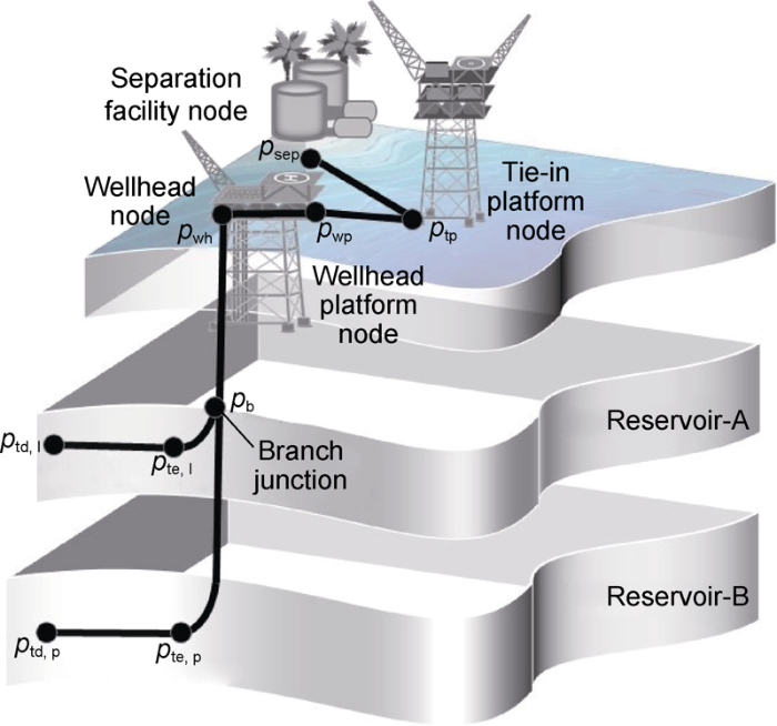
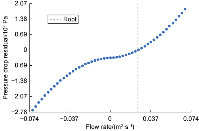
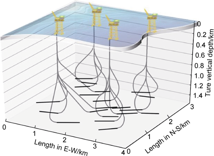
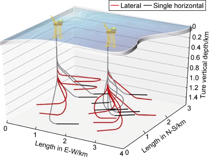
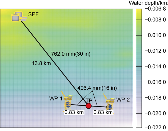

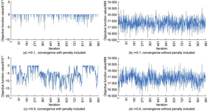

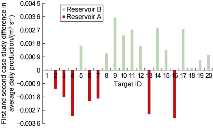
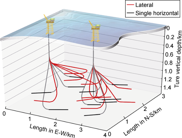
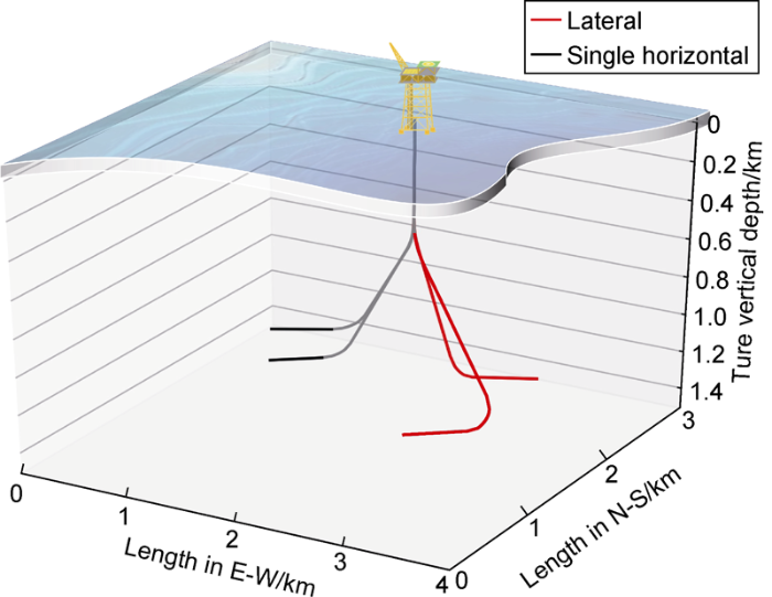
