


Introduction
Drilling is an essential key engineering technology for oil and gas exploration and development, and is also a very complex underground project. How to timely identify and deal with the safety risks while drilling, such as sticking, well wall instability and drilling tool fracture under complex on-site construction conditions, and prevent the occurrence of large accidents is the key part to improve the success rate and reduce the cost of drilling and completion [1]. At present, the identification of drilling risk during the drilling process mainly depends on people. The judgment results have strong subjectivity and time lag. It is difficult to accurately identify the risk on-site by people due to the vast differences in safety concerns between different well settings.
The intellectualization of oil and gas exploration and development has become a hot spot during the development of the global oil and gas industry and a revolutionary technology to ensure the security of energy strategy in China in recent years, with the rapid development of AI (artificial intelligence) technology in the world [2]. In 2015, Li et al. [3] established a relationship model between main risk factors during the gas drilling process, such as well wall instability, water production, gas production, downhole combustion and explosion, drill string failure, and corresponding parameter change, and developed an effective safety risk identification method based on existing surface monitoring technology. In 2017, Qiu et al. [4] analyzed seven factors affecting the downhole accident risk, such as drilling fluid density, rheology, fluid loss, rock type, and so on, and developed an assessment index system of downhole accident risk, and realized a fuzzy comprehensive quantitative assessment of downhole accident risk. In the same year, Guan et al. proposed a BP (error back propagation) neural network drilling risk assessment method based on the particle swarm optimization algorithm [5-6]. In 2020, Wang et al. [7] proposed a drilling model-expert system combination for identifying downhole safety risks. In summary, drilling technology is evolving from the traditional mode to a hybrid of machine learning and artificial intelligence [8]. At present, it is primarily concerned with expert systems combined with BP neural networks [9]. However, due to the limitation of experience and samples, there are only a few cases where real-time identification while drilling has been used successfully in drilling engineering.
To address the shortcomings of current intelligent drilling technology in sample collection, data preprocessing, and data feature extraction, in this study, we used the few-shot learning method to expand the sample data, and the convolution neural network, which is more effective for abstract feature extraction, to train and learn the monitoring data while drilling, in order to realize the extraction of implicit features of parameters. The convolution neural network structure model and training method were designed to match with the current monitoring data form while drilling, allowing for the intelligent identification of safety risks while drilling.
1. Characterization and related parameters of drilling safety risk
1.1. Monitoring parameters while drilling
Various monitoring instruments were used during drilling, and the data acquisition interval was typically 1-5 s. The monitoring data from a single well drilling in a single day exceeded 4×10⁴, which is a large and complex amount of data. The parameter variation characteristics of similar safety risks differ greatly during the drilling process under different well conditions. As shown in Fig. 1, when drilling into the production layer, the methane volume fraction and pipeline discharge pressure of Well A increased significantly, and the oxygen volume fraction decreased significantly. There was no obvious abnormality at the top drive speed and top drive torque. The methane volume fraction and pipeline drainage pressure of Well B increased slightly, and the oxygen volume fraction decreased slightly, but the top drive speed and top drive torque were abnormal due to induced sticking. If the field personnel do not have extensive experience, it is difficult to assess the safety risk of gas production in a timely and accurate manner using monitoring parameters while drilling. Therefore, intelligent safety risk identification methods with high identification accuracy and strong real-time performance are extremely important in drilling engineering.
Fig. 1.
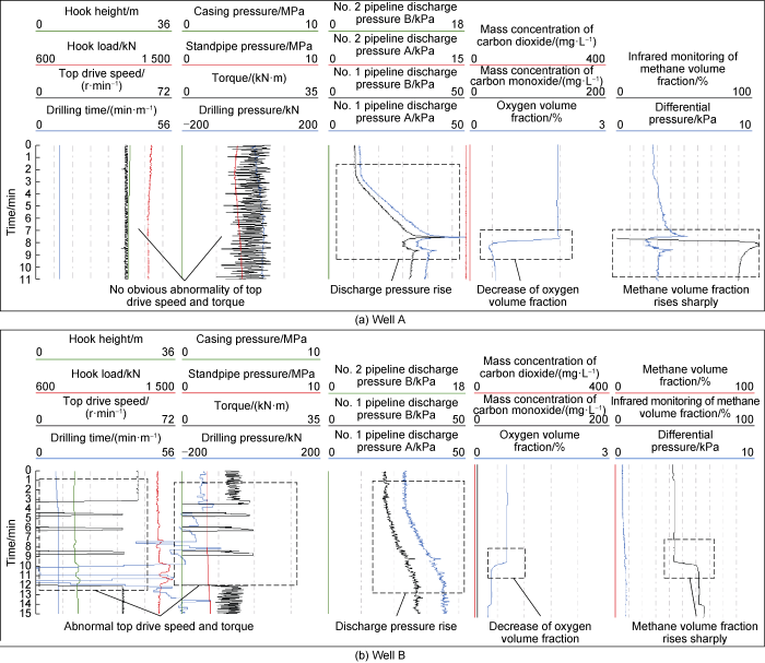
Fig. 1.
Schematic diagram of related parameter change in gas drilling process when encountering pay zones.
1.2. Correlation parameters for important safety risk characterization of gas drilling
With gas drilling as an example, significant drilling safety risks include formation gas production, formation water production, sticking, drilling tool fracture, downhole combustion and explosion, hydrogen sulfide production, well wall instability, and so on. Because of the various types of monitoring parameters while drilling, if all of them are used for safety risk analysis, the model complexity is high and the network training is difficult. Therefore, the corresponding relationship between safety risk and monitoring parameters while drilling must be controlled macroscopically. In this study, we collated and cleaned historical data from monitoring while drilling in more than 10 wells, and selected 13 core monitoring parameters for correlation coefficient analysis, which are shown in the form of a thermodynamic chart (Fig. 2). These figures show the correlation coefficients of the two corresponding parameters (including positive and negative correlation).
Fig. 2.
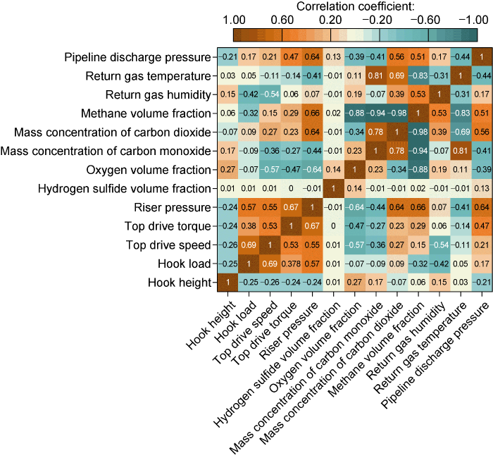
Fig. 2.
Pearson coefficient correlation analysis results.
The change laws of various safety risk data in the historical data were sorted out based on the correlation analysis results, combined with the existing safety risk while drilling theoretical model and the experience of multiple experts. The characteristic correlation parameters corresponding to some important safety risks are as follows: the related parameters of formation gas production risk are riser pressure, oxygen volume fraction, methane volume fraction, pipeline discharge pressure; formation water production risk related parameters are hook load, temperature and humidity of returned gas; sticking risk related parameters are top drive speed and top drive torque, riser pressure, pipeline discharge pressure; drilling tool fracture risk related parameters are hook load, top drive torque, riser pressure, pipeline discharge pressure; downhole combustion and explosion risk related parameters are riser pressure, oxygen volume fraction, mass concentration of carbon dioxide, methane volume fraction, return gas temperature, pipeline discharge pressure; well instability risk related parameters are hook load, top drive speed, and top drive torque.
2. Data sample of safety risk monitoring while drilling
Monitoring parameters while drilling are mostly collected in time order, and multiple parameters are stored in a two-dimensional array. The change trend of parameters in the two-dimensional array and the change relationship between parameters can effectively identify the majority of safety risks. Therefore, the sample structure of the intelligent security risk identification method should be a two-dimensional array composed of security risk characteristic correlation parameters over a period of time.
2.1. Time span analysis of sample
When converting monitoring data into neural network input data, it is necessary to determine the time span of a single sample. To address this issue, in this study, we constructed three different time-span sample data for each safety risk while drilling, conducted safety risk identification training while drill with three networks at the same time, and compared the performance, in order to ensure that the final sample form contains the majority of the characteristics of safety risk while drilling, improve identification reliability, and reduce the time delay of the system as much as possible. The time span distribution of the four types of safety risk samples is shown in Table 1, and the number of partial samples after construction is shown in Table 2. The sample library includes safety risk samples and normal drilling samples. The data in the second and third columns in the table are only the number of samples with security risk characteristics. Taking a sample with a formation gas production time span of 40 s as an example, the collection time interval is 2 s. Table 3 is a single sample after extraction, which is 20×5 two-dimensional data.
Table 1. Sample time span distribution
| Type of safety risk | 1# Sample time span/s | 2# Sample time span/s | 3# Sample time span/s |
|---|---|---|---|
| Formation gas production | 20 | 40 | 60 |
| Formation water production | 20 | 40 | 60 |
| Sticking drill tool | 20 | 40 | 60 |
| Connecting column | 120 | 150 | 180 |
Table 2. Number of partial safety risk samples while drilling
| Type of safety risk | Number of safety risk samples | Number of complete samples | ||||||||
|---|---|---|---|---|---|---|---|---|---|---|
| Training set | Test set | Training set | Test set | |||||||
| Formation gas production | 32 | 10 | 80 | 103 | ||||||
| Formation water production | 18 | 10 | 50 | 55 | ||||||
| Sticking drill tool | 22 | 10 | 50 | 53 | ||||||
| Connecting column | 26 | 10 | 70 | 72 | ||||||
Table 3. Schematic table of single sample
| No. | Formation gas production sample | Normal drilling sample | ||||||||
|---|---|---|---|---|---|---|---|---|---|---|
| Pipeline A discharge pressure/ kPa | Pipeline B discharge pressure/ kPa | Standpipe discharge pressure/ MPa | Methane volume fraction/ % | Oxygen volume fraction/ % | Pipeline A discharge pressure/ kPa | Pipeline B discharge pressure/ kPa | Standpipe discharge pressure/ MPa | Methane volume fraction/ % | Oxygen volume fraction/ % | |
| 1 | 35.98 | 30.50 | 2.08 | 75.63 | 1.27 | 12.43 | 10.48 | 2.44 | 0 | 3.29 |
| 2 | 36.23 | 30.55 | 2.32 | 84.30 | 0.93 | 12.48 | 10.55 | 2.45 | 0 | 3.29 |
| … | … | … | … | … | … | … | … | … | … | … |
| 19 | 37.10 | 31.63 | 2.64 | 94.24 | 0.12 | 12.28 | 10.33 | 2.44 | 0 | 3.29 |
| 20 | 37.53 | 31.70 | 2.83 | 93.39 | 0.11 | 12.28 | 10.38 | 2.44 | 0 | 3.29 |
Although the amount of monitoring data collected during drilling can exceed 4×10⁴ per well per day, there are few effective data segments that can characterize the occurrence of security risks, and the number of safety risk samples constructed is extremely limited. Furthermore, in order to avoid sample imbalance, the ratio of the number of samples with safety risk characteristics to the number of samples under normal working conditions should not exceed 1:2 in the sample library.
2.2. The safety risk identification while drilling by few-shot learning
If the sample size is fewer than 50, it falls under the few sample condition, according to British statistician William Sealy Gosset’s few-shot learning theory [10]. In this study, the sample database was created utilizing monitoring data from more than 10 wells and more than 20 times monitoring, resulting in a total of no more than 200 effective samples of four risks. Compared with the sample database with thousands of samples in other fields, the number of these samples are too less to efficiently extract the effective features of data by the network. As a result, in this study, we used the few-shot learning method to preprocess the sample data in order to increase the number of samples (Fig. 3). Under the condition of few samples, the data enhancement and transfer learning algorithms were mainly adopted in this study [11]. Scaling, clipping, interpolation, and the SMOTE algorithm [12] were used in data enhancement to increase the number of effective samples to a certain extent.
Fig. 3.
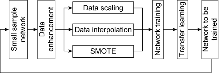
Fig. 3.
Schematic diagram of few-shot learning.
The mode of change of each monitoring parameter while drilling and the overall change law of parameters are more important than the value. Therefore, for some data segments with obvious change characteristics, the data scaling method can be used to extract and expand some data in the changing process to a standard time span (e.g., 20, 40, 60 s) in order to form new training samples. The scaled data segment is then filled with Lagrange piecewise interpolation [13] to make it the same data length as the standard sample:
Individual iconic samples are examined by the SMOTE algorithm after data scaling and interpolation, and new examples are artificially synthesized and added to the sample database to increase the network’s recognition performance. The following is the SMOTE synthesis algorithm [14]:
Table 4 shows the distribution of some safety risk training set samples and test set samples after the sample expansion. Compared with Table 2, the number of all kinds of samples has increased significantly. Furthermore, during network training, training preferentially the risk types with rich samples and obvious sample characteristics, such as formation gas production, and then use the migration learning algorithm [15] to migrate the trained network weight to the risk type training with less samples and unclear sample characteristics, such as formation water production, to improve the learning efficiency of the latter neural network [16]. In the migration process, if it is difficult to extract the features of a certain safety risk data sample, generally the hidden layer or output layer should be locked, and the convolutional layer (feature extraction layer) should be trained especially [17].
Table 4. Overview of some safety risk samples while drilling after sample expansion
| Type of Safety risk | Number of safety risk samples | Number of complete samples | ||
|---|---|---|---|---|
| Training set | Test set | Training set | Test set | |
| Formation gas production | 86 | 30 | 240 | 99 |
| Formation water production | 83 | 30 | 180 | 99 |
| Sticking drill tool | 79 | 30 | 200 | 99 |
| Connecting column | 84 | 30 | 160 | 83 |
2.3. Data normalization
Some parameters, on the other hand, must be normalized due to the large difference in the value range of monitoring parameters in the sample, which affects the network training effect. Methane volume fraction, oxygen volume fraction, and relative humidity are among the extracted parameters with values ranging from 0-100%.
Therefore, based on the above parameters, the other parameters are normalized within this range.
To summarize, the complete data sample construction method used in this study during the early stages of training are shown in Fig. 4. More than 10 wells in multiple blocks are included in the historical monitoring parameters, including Bozi Well A and Di Well A in Xinjiang, Dayi Well A in Sichuan, and Longgang Well A, etc. The sample source area span is large, the sample characteristics are diverse, and the similarities and differences between different well locations ensure the model’s generalization.
Fig. 4.
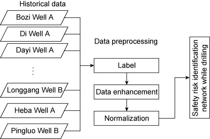
Fig. 4.
Schematic diagram of data preprocessing.
3. Convolution neural network for intelligent safety risk identification
The monitoring data samples during drilling can be considered as two-dimensional data. If the fully connected neural network commonly used in current data processing is used, and the input layer only supports one-dimensional data, all position relationships between the data will be lost [18]. In this study, we constructed a safety risk intelligent identification neural network structure based on the basic structure of convolution neural network input layer, convolution layer, excitation layer, hidden layer, and output layer, as well as the features of safety risk data samples (Fig. 5). To improve identification accuracy, time spans of 20, 40, and 60 s were chosen for a single sample of safety risk. At the same time, the data acquisition time interval of a single sample was 2 s to reduce the amount of system calculation and improve the efficiency and real-time performance of network identification. We made the last input layer data as 10×n, 20×n or 30×n two-dimensional matrix. It took a long time to reach the working condition of connecting column, which has an effect on the identification process. As a result, the working condition sample has a time span of 3 min, which is treated as a special case, and the input layer data is a 90×n two-dimensional matrix.
Fig. 5.
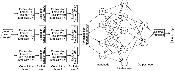
Fig. 5.
Structure diagram of convolution neural network for intelligent risk identification while drilling.
Multiple convolution kernels of different layers are frequently used to extract multiple features of input data in the process of feature extraction using convolution neural network, in order to improve the network's learning efficiency and generalization. The majority of the safety risk characteristics for the drilling construction process are primarily reflected in two aspects: (1) The change trend of each parameter. (2) The relationship between different parameters. In this study, with the convolution neural network model, we used two convolution layers for feature extraction, in order to fully extract the above two effective features of multiple monitoring parameters while drilling.
Because the input layer was a two-dimensional array of p×n (p = 10, 20, 30), and the elements in each column of the array were the time-varying values of the monitoring parameters while drilling, convolution layer 1 is responsible for extracting the change trend of each parameter. As a result, convolution layer 1 employs a one-dimensional longitudinal convolution kernel of m×1, and performs separate convolution calculations on n parameters. At the same time, the time span of parameter variation characteristics varied due to different safety risks. Convolution layer 1 employs convolution kernel of m×1 to check three types of time samples for operation in order to better integrate most safety risk characteristics. That is, separate feature extraction is performed for each parameter with multiple convolution kernels with different lengths. Table 5 shows the values of convolution kernel length m and moving step s used for samples with varying time spans. Multiple convolution kernels with the same m but different initial coefficients were used in the specific operation process, and each convolution kernel had different weight coefficients. This method extracts the features of the input data more thoroughly. As shown in Fig. 5, in convolution layer 1, a total of 20 convolution kernels were used.
Table 5. Values of parameters m and s in convolution layer 1
| Sample time span/s | m1 | m2 | m3 | s1 | s2 | s3 | |||
|---|---|---|---|---|---|---|---|---|---|
| 20 | 5 | 10 | No convolution kernel | 2 | 1 | No convolution kernel | |||
| 40 | 5 | 15 | 20 | 2 | 1 | 1 | |||
| 60 | 10 | 20 | 30 | 2 | 1 | 1 | |||
Following the processing of convolution layer 1, all elements in its output matrix were eigenvalues corresponding to the time progression of monitoring parameters. On this basis, the convolution layer 2 extracted the relationship between parameters by employing one-dimensional transverse convolution kernels of 1×n to check each row in the matrix for separate feature extraction, where “n” is the number of safety risk correlation parameters. The method for generating convolution kernels is similar to that of convolution layer 1. In convolution layer 2, we used a total of 20 convolution kernels, with a step size of 1.
Because 3 convolution kernels with varying lengths were used in convolution layer 1, and the characteristic data after convolution had at least three times the repetition characteristics, data dimensional reduction processing were used after convolution to reduce the data dimension to one-third of the original dimension, or the number of subsequent network input nodes increased greatly, reducing learning efficiency and convergence. This architecture used the principal component analysis method for dimension reduction [19] to obtain l eigenvalues, which were used as the input nodes of the conventional fully connected neural network, and a hidden layer with 150 nodes was used for learning and training. The activation function is identical to the ELU function. The output nodes take the form of dichotomy, with a total of two nodes. To facilitate quantitative description, the output layer employs the Softmax function to convert network output results into the probability of safety risk occurrence.
4. Neural network training results and field application
4.1. Training results and analysis of partial safety risk neural network
Samples with varying time span and safety risks were trained, and the training results were compared and analyzed in order to determine and validate the optimal sample time span and the performance of the convolution neural network [20]. The training set sample training and testing set sample testing were done concurrently.
4.1.1. Formation gas production risk network training
The sample of 20 s with small data volume were used to complete the neural network training process among the three samples with different time spans of formation gas production risk (Fig. 6).
Fig. 6.
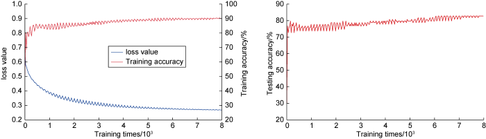
Fig. 6.
Training results of 20 s sample network for formation gas production risk.
The figure shows that after about 6000 times of training, the difference between the network model's output value and the real value (loss value) has been difficult to decrease, the training accuracy of the entire training set basically does not rise after reaching 90%, and the testing accuracy of the test set is only about 83%. Furthermore, the accuracy change trend of the two types of samples during the training process is not completely consistent, indicating that it is difficult to fully show the change law and characteristics of formation gas production risk in 20 s. The sample with 20 s contains fewer effective data characteristics, resulting in over-fitting in network learning. As a result, sample with this length cannot be used to identify formation gas production risks.
The data volume of 40 s and 60 s samples is large, the data characteristics contained in the samples are diverse, and the final training effect is improved. Fig. 7 shows that after 7000 times of training of samples with 60 s, the final loss value is less than 0.1 and the accuracy of the training and testing sets is greater than 95%.
Fig. 7.
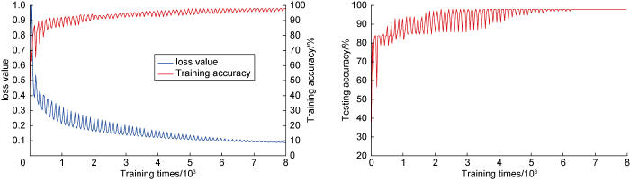
Fig. 7.
Training results of 60 s sample network for formation gas production.
4.1.2. Formation water production risk network training
After training about 5000 times for 3 samples of time in the formation water production risk network training process, the loss value and accuracy were stable. Similar to formation gas production samples, increasing the time span of a single sample of formation water production enriched the data characteristics contained in the samples and improved the network training effect. Finally, the network recognition accuracy of 60 s samples was the highest, as illustrated in Fig. 8. The accuracy change trend of the training set was essentially synchronous with that of the test set, and was also very close in size, basically eliminating the possibility of over-fitting. However, because of the small number of samples obtained on-site under this risk condition, the final accuracy of the test set was slightly lower, reaching only 87%. Following that, increasing the number of risk samples can be used to improve the accuracy even further.
Fig. 8.
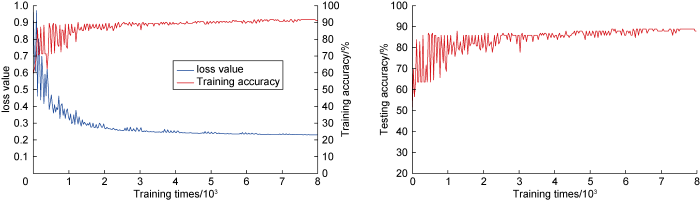
Fig. 8.
Training results of 60 s sample network for formation water production risk.
4.1.3. Sticking risk network training
During the process of network training, the samples of 40 s and 60 s of sticking risk converged rapidly, the loss value decreased rapidly, and the accuracy of the final training set was nearly identical to that of the test set. The training results of 60 s sample are shown in Fig. 9. It can be seen that after about 1000 times of training, the loss value is less than 0.1, the accuracy of the training set is greater than 95% and eventually close to 99%, and the accuracy of the test set reaches 90% and tends to be stable.
Fig. 9.
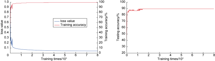
Fig. 9.
Training results of 60 s sample network for sticking risk.
The final accuracy of the neural network test set corresponding to the three safety risks of 60 s samples is 95%, 87%, and 90%, respectively, and the identification accuracy is close to or greater than 90%, indicating that the intelligent identification method has a good identification effect in drilling safety risk identification and can meet the requirements for intelligent identification. The identification network training converges quickly, especially for the sticking risk, demonstrating that for this convolution neural network structure, the network can easily extract and learn effective features, achieve efficient identification and prediction, avoid or quickly solve the drilling on-site risk, and fully realize the applicability of convolution neural network architecture in the field of intelligent drilling. Furthermore, the model’s generalization and identification accuracy can be improved by increasing the number of samples.
4.2. Field application
The intelligent identification and warning software system of safety risk while drilling in gas drilling was compiled after integrating all of the trained neural network models, and many on-site identification and warning applications were carried out.
Several times of formation gas production, formation water production, sticking risk, and column connection conditions were successfully identified in Dayi Well A. When the on-site drilling construction reached the measured well depth of 5149.22 m, the identification system notifies that the probability of formation gas production has reached 97.25%. The on-site monitoring personnel then confirmed the presence of a small stream of methane gas while drilling, while the system successfully identified the risk. The identification system reminds that the probability of formation water production is 83.54% when drilling to the measured well depth of 5254.58 m. The on-site monitoring personnel reported to the decision-maker and confirmed that the drilling encountered the water layer based on the subsequent sand discharge status, so the system successfully warned of the risk; when drilling to the measured well depth of 5254.69 m, the identification system reminded that the sticking probability was 96.54%. The on-site monitoring personnel then conformed that the occurrence of sticking problem and notified the driller for treatment. The risk was successfully identified once more by the system. After the drilling construction was completed, the system intelligent identification results were compared to the expert conclusions in the monitoring report while drilling, and the results were consistent (Table 6).
Table 6. Comparison between identification results and monitoring results in Dayi Well A
| Well depth/m | Monitoring report and expert conclusion | Risks produce probabilistic of intelligent identification results/% | |||
|---|---|---|---|---|---|
| Formation gas production | Formation water production | Sticking | Connecting column | ||
| 5149.22 | Formation gas production | 97.25 | 1.71 | 0 | 0 |
| 5173.06 | Connecting column | 0.14 | 1.58 | 0 | 99.44 |
| 5174.45 | Formation gas production | 99.34 | 1.78 | 0 | 0 |
| 5133.02 | Connecting column | 0.96 | 2.61 | 0.02 | 99.98 |
| 5250.62 | Formation gas production and sticking | 98.80 | 46.13 | 99.92 | 0 |
| 5251.64 | Formation water production | 3.48 | 85.34 | 2.22 | 0 |
| 5254.58 | Formation water production | 4.15 | 83.54 | 0 | 0 |
| 5254.69 | Sticking drill | 1.52 | 29.02 | 96.54 | 0 |
5. Conclusions
Compared with the traditional BP type fully connected neural network architecture, the monitoring while drilling data sample establishment method designed in this study, as well as the convolution neural network structure and its training method matching the sample data form, can more deeply and effectively perceive the abstract change law and hidden correlation of multiple monitoring while drilling parameters during the drilling process, and effectively identify the safety risk. To some extent, the gas drilling safety risk intelligent identification system built on this foundation can basically solve the problems of few safety risk samples and low intelligence in the drilling field. Many field applications have demonstrated that the identification accuracy of various safety risks while drilling in the process of gas drilling construction is approximately 90%, which is very practicable.
Nomenclature
A—input node;
B1, B2—output node;
H—hidden layer node;
i—the No. of the first existing sample participating in the calculation;
j—the No. of the second existing sample participating in the calculation;
l—total number of input nodes (main characteristic dimension);
m1, m2, m3—vertical length of convolution kernels 1-1, 1-2, 1-3;
n—number of characteristic parameters of various safety risks;
p—longitudinal length of sample;
q—the total number of sample points involved in the calculation;
r—number of hidden layer nodes;
rand(0,1)—random number in interval [0,1];
s1, s2, s3—convolution kernels 1-1, 1-2, 1-3 convolution process moving step size;
u—abscissa value of insertion point;
vi—ordinate value of existing samples;
ui, uj—abscissa value of existing samples;
Vq(u)—output ordinate value by interpolation method;
(x, y)—original sample points;
(xnew, ynew)—new sample points;
(xn, yn)—nearest neighbor of original sample point.
Reference
Key technologies and practice for gas field storage facility construction of complex geological conditions in China
Application and development trend of artificial intelligence in petroleum exploration and development
DOI:10.1016/S1876-3804(21)60001-0 URL
While-drilling safety risk identification and monitoring in air drilling
Study on fuzzy evaluation of downhole drilling accident risks and application
Dynamic risk assessment method of drilling based on PSO optimized BP neural network
A quantitative evaluation method of drilling risks based on uncertainty analysis theory
Real-time intelligent drilling monitoring technique based on the coupling of drilling model and artificial intelligence
Real-time intelligent identification method under drilling conditions based on support vector machine
Survey of few-shot learning based on deep neural network
Data augmentation method based on generative adversarial networks for facial expression recognition sets
On data augmentation for GAN training
DOI:10.1109/TIP.2021.3049346 URL [Cited within: 1]
Regularization graph convolutional networks with data augmentation
DOI:10.1016/j.neucom.2020.12.124 URL [Cited within: 1]
SMOTE: Synthetic minority over-sampling technique
DOI:10.1613/jair.953 URL [Cited within: 1]
Survey on transfer learning research
Automatic fault recognition with residual network and transfer learning
A comprehensive survey on transfer learning
DOI:10.1109/JPROC.2020.3004555 URL [Cited within: 1]
Review of convolutional neural network
Log facies recognition based on convolutional neural network
Automatic well test interpretation based on convolutional neural network for a radial composite reservoir
